
Key takeaways
- Memory is your model's size: Optimizing it is key to refresh and query performance for reports, Copilot, and data agents.
- Memory limits are hard ceilings: Power BI Pro, PPU, and Fabric enforce per-model memory limits, and unlike compute they aren't flexible or adaptive.
- Refresh needs extra memory: A full import refresh can require two copies of the model plus overhead, so a model that fits at rest can still fail during refresh.
- Changing storage mode isn't a fix: Import, Direct Lake, and DirectQuery shift memory costs differently, but none make memory constraints disappear.
- VertiPaq Analyzer finds the cause: It's the fastest way to go from "my model is too big" to "this specific column is the problem."
What is “semantic model memory” and why is it important?
Memory refers to how much space your semantic model takes up. Larger models have a bigger “memory footprint”; there’s more data. This is a common challenge for almost every organization who uses Power BI and Fabric, since there’s a limit for how big memory can be.
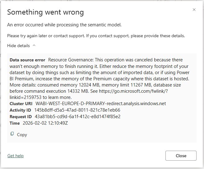
If you exceed this memory limit, then refreshes fail with the error: An error occurred while processing the semantic model… Resource Governance: This operation was cancelled because there wasn’t enough memory to finish running it. If you get this error, then you must either reduce the semantic model’s memory footprint with optimization or upgrade your Power BI license or Fabric capacity SKU.
Optimizing your semantic model memory is always the first step, and it brings the following benefits:
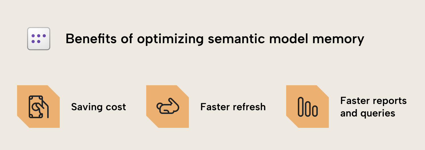
- Saving cost: If you keep models small, you don’t have to upgrade your license or Fabric SKU for higher limits. For DirectQuery models, this also means cheaper queries. This also applies for Direct Lake, which has the same guardrails around total model memory.
- Faster refresh: Many of the actions you take to optimize memory often also help to improve your refresh times.
- Faster reports and queries: Smaller models usually perform better in general, not just when it comes to refresh but also DAX queries from reports, Copilot, and data agents.
This article is the first in a three-part series on optimizing semantic model memory in Microsoft Fabric. All examples are based on a reproducible lab environment built on the NYC Yellow Taxi dataset. You can use this environment to follow along and apply these techniques for yourself.
The goal of this first post is to help you understand memory limits in Fabric, and why it’s still predictable. Specifically, what you get with a Fabric SKU, why refreshes can fail even when models appear to fit, how storage modes change the picture, and how to measure where memory is going before touching model design. Then, in later posts, we’ll teach you the best techniques to do this optimization for your models.
NOTE
Memory is correlated with, but not identical to, the size of your Power BI Desktop (.pbix) files; the model on disk. Memory is the VertiPaq-compressed data loaded into RAM, while on-disk size is usually smaller; it’s the same data compressed further for storage. A .pbix file might also contain other supporting files or report metadata, which isn’t relevant for VertiPaq memory. A PBIP file might also contain a cache.abf, with a local cached copy of the model and data.
Why semantic model memory is still hard
Optimizing model memory is nothing new. It’s an ongoing challenge since the VertiPaq engine first appeared as Power Pivot in Excel 2010, and later in Analysis Services Tabular and Power BI datasets / semantic models. In Microsoft Fabric, only the environment around the engine has changed:
- Capacity-based governance
- Direct Lake as a first-class option
- SKU-based memory limits
The model is clear on paper, but in practice, it’s still easy (and common) to hit your memory limits.
NOTE
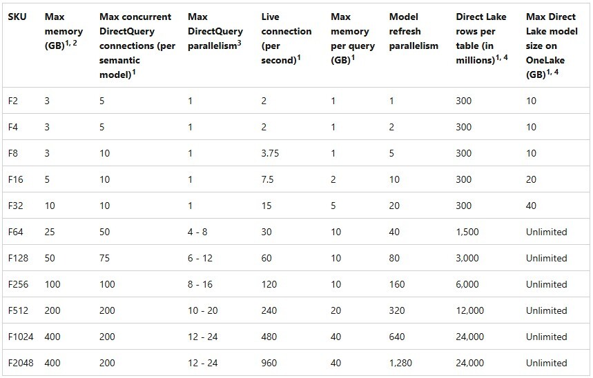
Optimizing semantic model memory isn’t a problem exclusive to Microsoft Fabric, where it’s determined depending on the Fabric SKU that you have (for example, limits like 3 GB for F2 SKU or 25 GB for F64 SKU). It’s a cost challenge on any platform; you pay for RAM, directly or indirectly.
Memory limits for semantic models also exist in Power BI Premium (25 GB) and Power BI Pro (1 GB).
Memory vs. compute in Microsoft Fabric
Before we continue, it’s important to understand two different things: compute and memory. In Fabric, compute and memory can be understood as follows:
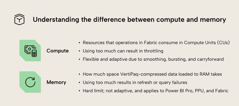
- Compute is a measure of the resources that operations in a Fabric capacity consume, measured in Compute Units, or Compute Units seconds (CUs). It ultimately maps to time on a CPU. When you use too much, you can experience throttling, which is when you experience degraded performance of operations like refreshing or querying a semantic model. Compute is flexible, since Fabric can smooth, burst, and temporarily run above your nominal CU budget (i.e. with overages and carryforward) before throttling kicks in. That’s why short spikes during refresh or interactive peaks can still succeed without you experiencing the pains of overuse, right away.
- Memory is a hard ceiling, the maximum size for a semantic model. It ultimately maps to space in RAM. Furthermore, unlike compute, memory is not flexible; if you exceed the memory limit, then semantic model refreshes will fail and you won’t see up-to-date data in downstream queries from Copilot, data agents, and reports. As we mentioned above, memory is relevant not only in Fabric, but also in Power BI Pro and Premium-Per User.
Microsoft documents the semantic model limits per Fabric SKU in detail, including memory, refresh parallelism, and Direct Lake constraints:
NOTE
Memory limits are enforced per semantic model. This is a big mental shift if you come from Azure Analysis Services or SQL Server Analysis Services, where models compete for shared server memory. In Power BI and Fabric, one large semantic model that exceeds the limit will fail to refresh.
It’s worth noting that the optimizations discussed here are for reducing the compressed size of columnstore data. It applies to the size on disk in OneLake, because that is Parquet… also columnstore compressed data.
When considering the above limitations, a common trap is to look at the advertised “Max memory (GB)” and assume a model of that size should fit. In practice, you almost always need meaningful headroom; the memory limit isn't only about the final model sitting in memory, but also refresh behaviour, query execution, and other, internal overhead. Chris Webb’s series on memory errors is a good reference point for how these limits surface and why the errors are deterministic rather than “service flukes.”
When a semantic model is “too big” and it no longer fits in memory, scaling the Fabric capacity is technically the easiest and most obvious option… but it’s also the most expensive. Memory upgrades are not granular. For example, moving from an F8 (3 GB) to the next available memory tier means jumping straight to an F64 with 25 GB… which is far more than a simple doubling in cost. This becomes even more complicated if you run aground with size limitations in Power BI Pro or PPU, since this could mean implementing or migrating to Fabric (or another platform) and all the adoption, architecture, and governance decisions that come along with it.
Understanding the semantic model memory model in Fabric
The single most important behaviour to internalize is how Import mode refresh works.
Why full refresh needs more memory than you think
In Import mode, a full refresh doesn't overwrite the existing model in place. Instead, the engine builds the refreshed model side-by-side, and only when processing completes successfully does it swap to the new version. That is great for end users, because queries can continue while the refresh is running. The trade-off is that refresh is memory-hungry.
During refresh, you should expect memory to be consumed by operations such as:
- The current in-memory model
- The new model being processed in parallel
- Processing overhead (encoding, dictionaries, internal structures)
- Query memory for concurrent report usage
WARNING
A model that “fits” after refresh can still fail during refresh. Retrying will not fix it; the operation is failing deterministically due to insufficient memory headroom.
You can see this demonstrated in the following diagram:
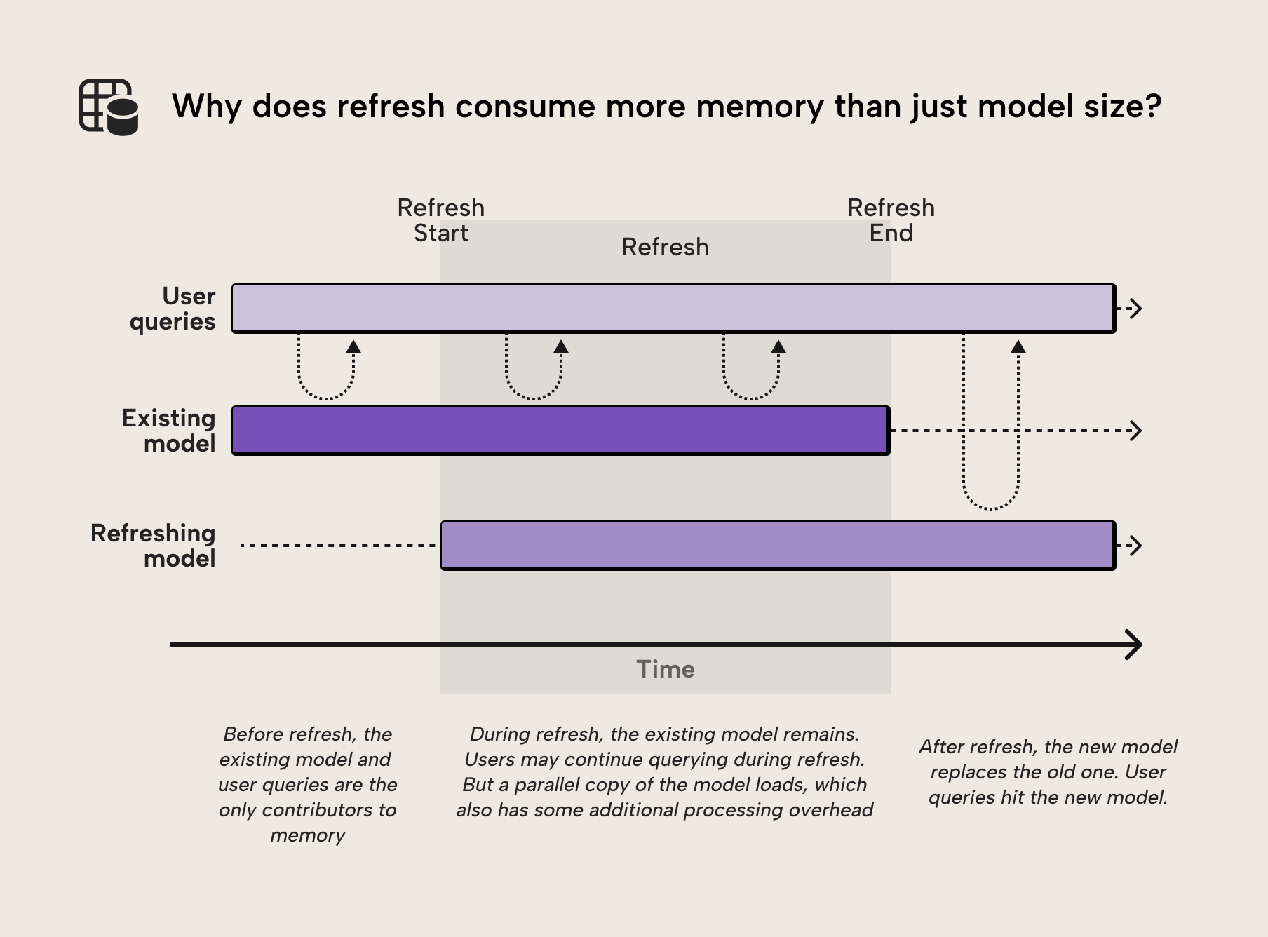
The result is that at the time of refresh completion, the total memory consumption is the sum of user queries, processing overhead, and both the pre-refresh and post-refresh model:
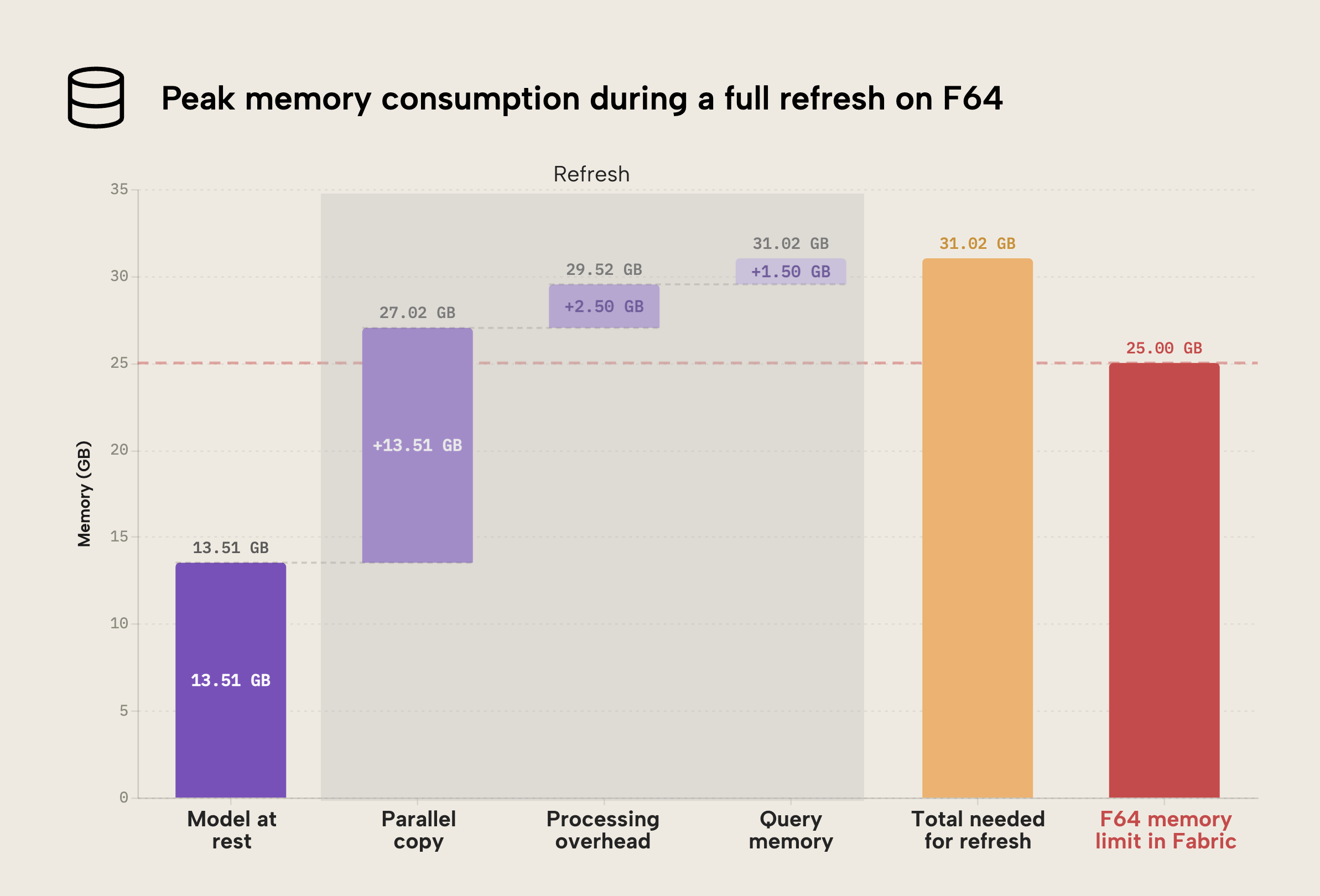
- At rest, the model is 13.51 GB.
- During refresh, the new model (“parallel copy”) is processed in parallel. This consumes another 13.51 GB. Already, we are over the 25 GB limit of Fabric. Note that the new model is likely not the same size as the old, pre-refresh model; it’s just depicted as such here for illustrative purposes. It could be smaller (if there’s less data) or larger (if there’s more) than the pre-refresh model.
- There’s some additional processing overhead, shown here as 2.50 GB.
- Concurrent user queries can have an additional impact, shown here as 1.50 GB.
- The total memory footprint of the model during refresh would thus be 31.02 GB, and a memory limit above this number would be required for the model refresh to complete successfully.
TIP
If your model is only failing because of refresh processes and not its total size, a quick fix can be to refresh individual tables or partitions one (or a few) at a time using Tabular Editor, other XMLA tools, or APIs. When refreshing one table, you only need memory headroom sufficient for a second copy of the table, instead of a second copy of the whole model. Refreshing individual objects doesn't change the formula, just the scale you are operating at.
Note that this doesn’t fix your problem; it limits the refresh operations to a subset of your model.
The error message often looks surprising at first, because the reported model size appears well below the SKU limit. Once you account for the side-by-side refresh behavior and processing overhead, the failure becomes predictable rather than mysterious.
Full refresh is the default behavior for Import models, but it’s not the only option. Partial refresh techniques, such as Incremental Refresh and custom partitioning, can significantly reduce refresh-time memory requirements by limiting how much data is refreshed at once. These approaches introduce additional design considerations; we cover them in a later post in this series.
TIP
If your model refreshed fine at first, but suddenly started failing later, this might be due to data growth (more rows, more history, more detail). In this case, assume that the problem is due to “lost headroom”, first. Before scaling capacity, validate what changed in model size and which columns drove it.
The simplest way to solve the problem is with additional filtering or removing columns that you don’t need (because they aren’t used downstream in DAX, relationships, or reports).
Storage modes and their memory implications
Storage modes are often discussed as memory fixes that let you fit more data into Power BI… but they’re not. They’re trade-offs. Choosing between storage modes in Power BI is a deliberate decision that must be made carefully.
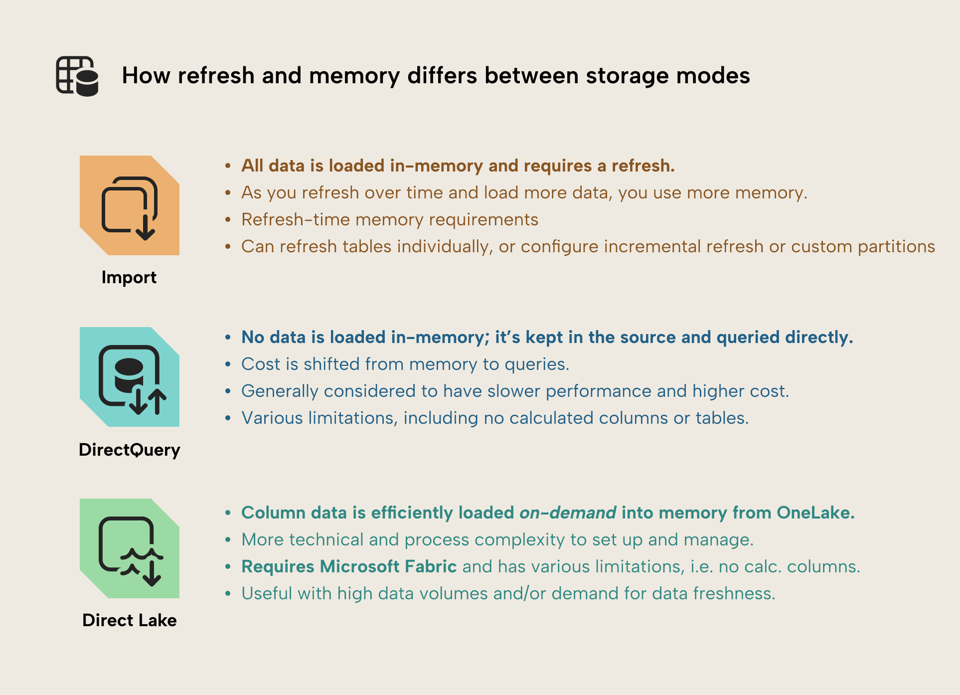
The following diagram and sections give you a concise overview:
Import mode
Import gives you the best query performance, but you pay predictable, steady memory usage. Over time, as you refresh, you load more data if data volume grows, which uses more memory. Most optimization patterns assume Import is the default starting point, since it’s still the preferred default suitable for most scenarios. Size optimization applies to all models, however.
NOTE
If filters constrain data to a fixed-size time window or scope, you might not see memory increases with import. One way to do this is with fixed filters, but also with incremental refresh.
Direct Lake
Direct Lake changes the refresh story because data is read directly from OneLake and transcoded into memory on demand. This can reduce refresh-related memory spikes, but it doesn't eliminate memory usage. Memory is still consumed when columns are accessed, and query patterns matter. Once the column data is available for DAX queries, it is exactly the same VertiPaq storage engine as with Import mode models; the only difference is the process by which the data is loaded into memory.
There is also a modest but real performance cost. When data is accessed for the first time, refresh is slower; data must be read and transcoded before queries can execute. This initial latency is usually acceptable, but it should be understood rather than assumed away.
NOTE
There are also data management and orchestration requirements that Direct Lake requires, which import mostly just deals with for you. For instance, data fragmentation due to small writes or updates can lead to worse performance characteristics. This can be complex, but Microsoft has written good documentation about this.
DirectQuery
DirectQuery minimizes semantic model memory usage because data isn't imported into VertiPaq. Instead, the model primarily contains metadata. The cost is shifted to query latency, source system load, and often increased CUs. It is a valid design choice, but not a free optimization.
NOTE
Storage modes do not remove memory constraints. They change when and how memory is consumed, and they usually move pressure to a different part of the system (source performance, CU usage, query latency, or all three).
Again, for a structured overview of storage modes and when they make sense in Power BI and Fabric, see the Tabular Editor article on semantic model types.
Where semantic model size comes from
Row count isn't a reliable predictor of model size; you can have a Power BI semantic model that contains hundreds of millions of rows, but is still smaller than a model with hundreds of thousands of rows. That’s because VertiPaq stores data column-by-column, and compression behavior is shaped by dictionaries, cardinality, and encoding.
At a high level, VertiPaq creates a dictionary of unique values for each column and stores the column as references into that dictionary. Columns with many unique values tend to build large dictionaries, and those dictionaries can dominate model size. This is very common when you have columns like primary keys, document identifiers, long strings, and values that have high-precision decimals.
This is why “one innocent column” can end up consuming a shocking share of memory. A high-cardinality datetime column is another classic example: it looks harmless, but it can create an enormous dictionary if it is near-unique per row. This is why it’s so important to be able to view and inspect the memory usage per semantic model object.
For a deeper explanation of how VertiPaq compression works and how dictionaries, cardinality, and encoding interact, this article by Data Mozart provides an excellent conceptual overview.
Inspecting model memory with VertiPaq Analyzer
Before you optimize, you need to see. The VertiPaq Analyzer is still the best and fastest tool for that job. It’s a tool from SQLBI designed to analyze VertiPaq storage structures and report size breakdowns at model/table/column level. Today it is also integrated into tools like Tabular Editor, which makes it a natural part of the modeling workflow.
At this stage, the goal isn't to “fix” anything. The goal is to be able to point at a model and say: “This is where memory goes.” That is what turns optimization into engineering instead of guesswork.
NOTE
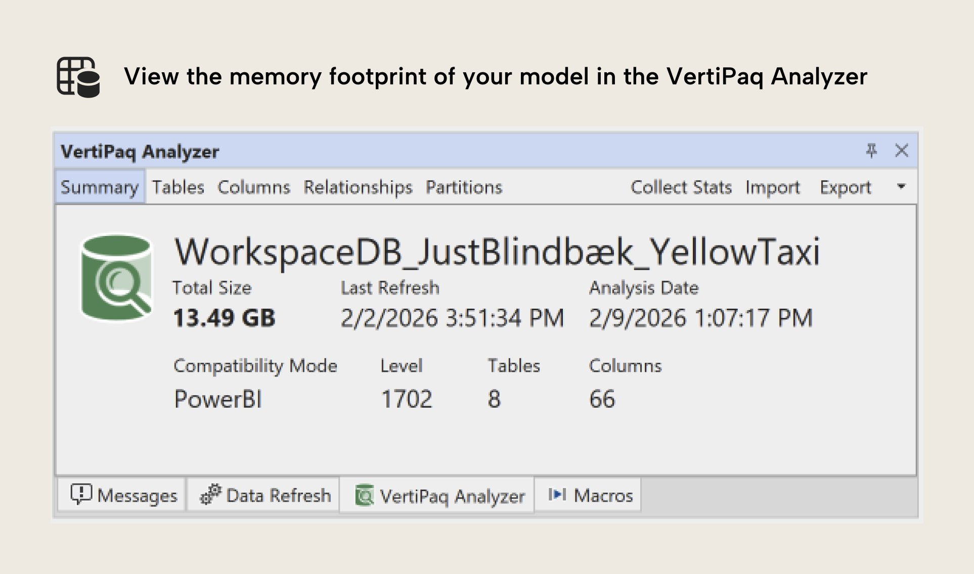
To reiterate, this number (13.49 GB) isn't the same as the size on-disk of the model in a PBIX file. Usually, the “total size” in memory is larger, because the PBIX is further compressed for file storage.
A simple inspection workflow involves:
- Run the VertiPaq Analyzer
- Go to the Columns view
- Sort by % of DB size (or total size)
- Identify the top offenders and what drives them (dictionary size vs data size)
The following table shows you an example of a VertiPaq Analyzer result, where you can view, sort, and save the memory statistics for your semantic model:
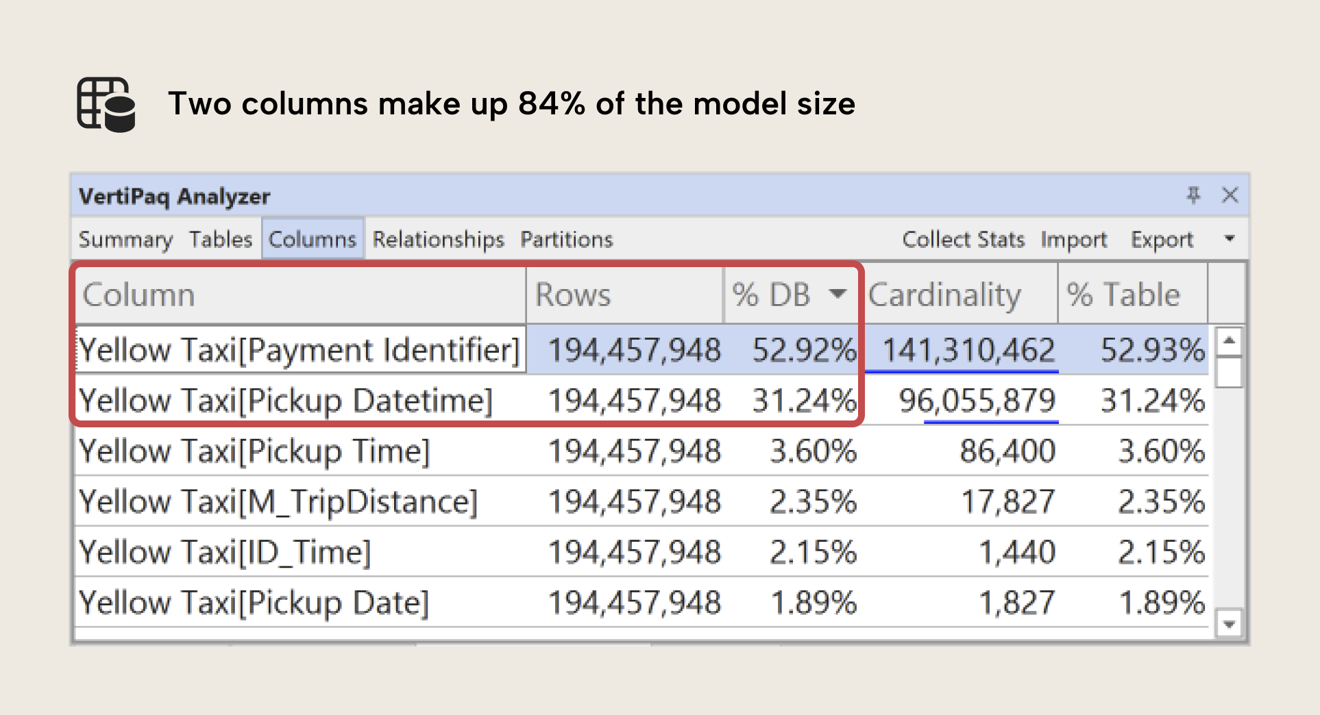
In this example using our sample dataset, we can clearly see that the highest fields are Payment Identifier and Pickup Datetime, which together take up ±84% of the total model size. In the next article, we’ll demonstrate what you do in these scenarios to optimize the design and size of your semantic model so this doesn’t happen.
NOTE
VertiPaq Analyzer doesn't provide any meaningful data with a DirectQuery model. It’ll also only show size information about columns that haven't been paged out to disk for Direct Lake models. If you want to understand a Direct Lake model in whole, you probably need to write a C# script, DAX query, or notebook to query every column in the model, so that all columns are all transcoded from disk.
Semantic model memory summary
So, wrapping up, at this point, you should be able to:
- Understand that memory reflects the size of your semantic model and how much data is in it. This is the VertiPaq-compressed data.
- Recognize that Power BI Pro, PPU, and Fabric have hard memory limits, and exceeding these limits results in refresh failures. High memory results in large models, which are typically slower to refresh and use, and expensive to query.
- Know that when you run into issues with memory you should start with optimization before you consider upgrading your Power BI license or Fabric SKU.
- Understand that memory limits are per semantic model, and that memory is required not just for latent data, but also other operations relevant during the refresh of your semantic model. You thus need to reserve “extra space” for these operations.
- Understand why refresh errors and memory limits aren’t solved by changing the semantic model storage mode, since the cost isn't reduced, just shifted elsewhere.
- Know how to view model memory usage by using the VertiPaq Analyzer, which shows the total memory so you can identify which tables, columns, and relationships are consuming the most space.
TIP
If you want a broader checklist mindset, this semantic model checklist is a useful companion reference.
For further reading
- Optimizing semantic model size in Power BI and Fabric: a comprehensive guide (Tabular Editor). The next article in this series, covering six concrete patterns to shrink the model's footprint once you understand where memory is going.
- Optimizing semantic model refresh memory in Power BI (Tabular Editor). The third part of this series, focusing on peak memory during processing rather than steady-state size.
- Storage analysis tool documentation (SQLBI). Covers the VertiPaq Analyzer output used here to inspect model memory at model, table, and column level.
- Configure incremental refresh and real-time data for Power BI semantic models (Microsoft Learn). Official reference for the partition-based refresh approach mentioned as a workaround for refresh-time memory pressure.
In conclusion
In the next post, we will apply concrete, measurable memory optimization patterns to help you reduce the size of your semantic models.
Reduce Fabric semantic model memory with a clearer Tabular Editor 3 workflow.
Give Tabular Editor a spin