When DAX UDF measures beat calculation groups for time intelligence

Key Takeaways

• The paradigm has changed. For scenarios with moderate to high complexity of requirements, time intelligence measures with DAX UDFs are easier to use than calculation groups, while keeping logic centralized as well.
• C# scripts that empower DAX UDFs. Even when using DAX UDFs, creating the necessary measures, field parameters, and dynamic measures to cover most reporting requirements is time-consuming if done manually. Publicly available scripts can automate the process.
• Calculation groups leak into tooltips, titles, and filter panes. When a calc-group column lives in a slicer or legend, it affects every measure under that filter context — dynamic titles can error out, tooltip pages get filtered the same way the chart is, and measure-value filters lose what they should be showing. DAX UDF measures stay invisible to the report, so the leak doesn’t happen.
• Calculation groups still have their place. Role-playing dimensions via USERELATIONSHIP, TREATAS for impossible relationships, and a handful of DAX-fusion edge cases continue to be cleanly served by calc groups — this article focuses on the scenarios where UDF measures are the better choice.

This summary is produced by the author, and not by AI.

Ever since DAX UDFs came out as public preview in September 2025, many DAX developers started wondering how they will compare with calculation groups since both have the centralization of code as one of their main selling points. As pointed out in a recent article by SQLBI they are indeed very different beasts, even though they can be used to achieve very similar outputs.

In short, a calculation group is a model-level object whose items swap one DAX expression for another at evaluation time. Once an item is in the filter context, it applies to every measure being evaluated. A DAX UDF is a smaller object: a named, reusable expression with parameters, callable from any measure but invisible to report users.

The key distinction is that a calculation item applies whenever it is part of the filter context, regardless of what any measure does. A DAX UDF runs only when a measure’s expression explicitly calls it. Both centralize logic. While calculation groups are still the best approach for some use cases, this article focuses on the scenarios where DAX UDF measures are the better choice instead.

Let’s check in detail some of the aspects that make calculation groups difficult to use for model developers and report creators, and how to use DAX UDF measures in such scenarios.

Limiting the impact

Limiting the impact of a calculation item is probably one of the trickiest elements to consider when working with calculation groups. When a calculation item is applied at the visual level, all measures in the visual are affected without exception. The expression of the calculation item replaces the expression of the measure, which may or may not include a reference to the original measure (via SELECTEDMEASURE). This is how they work.

For simple time intelligence calculations, there’s no need to bother too much. Applying a filter on all measures to show previous-year values will not break anything (even though it will apply to the title which may or may not be what you want).

// Dynamic title measure
Sales Year = "Sales of " & SELECTEDVALUE('Date'[Year])

// Calculation item
PY = CALCULATE( SELECTEDMEASURE( ), DATEADD( 'Date'[Date], -1, YEAR ) )

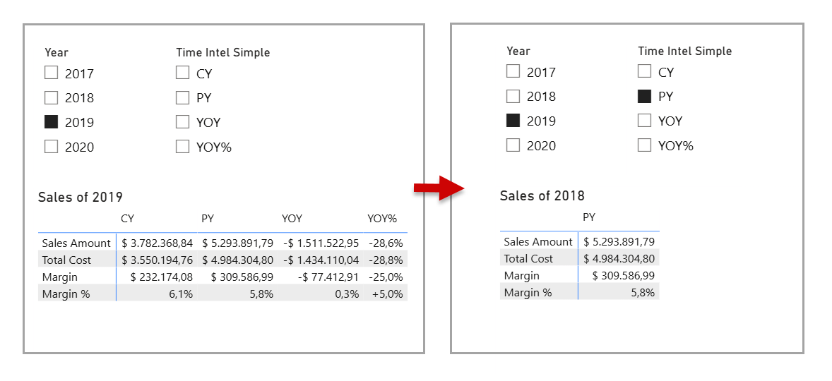
The title is also affected by the calculation item

However, other popular time intelligence calculations such as year-over-year can have more dramatic consequences.

CALCULATIONITEM "YOY" =
    VAR _cy = SELECTEDMEASURE( )
    VAR _py = CALCULATE( SELECTEDMEASURE( ), DATEADD( 'Date'[Date], -1, YEAR ) )
    RETURN 
        IF( 
            ISBLANK( _cy ) || ISBLANK( _py ), 
            BLANK( ), 
            _cy - _py // If the measure is text, this will fail
        )

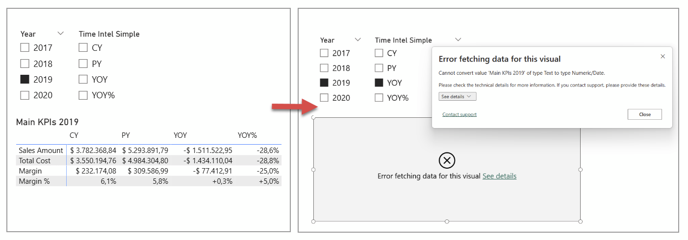
Due to the interaction of the calculation group and the dynamic title, the visual crashes

If you are using dynamic titles, or conditional formatting by field value, you need to pay attention. The moment a calculation item expression with a subtraction (such as in year-over-year) replaces text measures, the visual will crash as it’s not possible to subtract text values. In the example above, we end up evaluating the dynamic title measure for the current year and the prior year; this ends up trying to do "Sales of 2019" - "Sales of 2018", literally subtracting one string from another. Also, the calculation may also impact other measures used for cosmetic purposes with numeric values. As we will see later in this article, even for regular base measures, sometimes we want to suppress the calculation item logic, and this poses a challenge.

Of course, as any savvy reader will know, calculation groups were released with some DAX functions to deal with such situations. ISSELECTEDMEASURE and SELECTEDMEASURENAME allow us to create a necessary conditional expression to apply the year-over-year calculation only for certain measures, while leaving the rest as-if nothing changed, using the SELECTEDMEASURE placeholder. Recently, new DAX functions such as ISTEXT can also help us on this front. In other words, to prevent errors in the report, you need to move from expressions like this:

VAR _cy = SELECTEDMEASURE( )
VAR _py =
    CALCULATE(
        SELECTEDMEASURE( ),
        SAMEPERIODLASTYEAR( 'Date'[Date] )
    )
VAR _result =
    IF(
        ISBLANK( _cy ) || ISBLANK( _py ),
        BLANK( ),
        DIVIDE( _cy - _py, _py )
    )
RETURN
    _result

To expressions like this:

IF(
    ISTEXT(SELECTEDMEASURE()), 	 // If the value is text,
    SELECTEDMEASURE(),		     // leave it unchanged,
    VAR _cy = SELECTEDMEASURE()  // otherwise apply yoy calculation
    VAR _py =
    CALCULATE(
        SELECTEDMEASURE(),
        SAMEPERIODLASTYEAR( 'Date'[Date] )
    )
    VAR _result =
    IF(
        ISBLANK( _cy ) || ISBLANK( _py ),
        BLANK(),
        DIVIDE( _cy - _py, _py )
    )
    RETURN
    _result
)

A subtle catch: ISTEXT(SELECTEDMEASURE()) returns FALSE for BLANK(), so measures that can return either text or blank still slip through this guard and trigger the year-over-year branch.

However, this is just one simple example. For medium to large models (in terms of measures and calculations required), the logic defining which measures should be modified by the calculation can grow more complex, increasing the burden of maintenance. And even if all this logic was easy to maintain, it does not make much sense to evaluate all this impact logic at query time when it’s something that should be “hard-wired”.

In contrast, with DAX UDF measures, there’s no need to “limit the impact” at all. Measures requiring certain logic will include in their expression the call to the corresponding function, whereas the rest will not. Using a measure with year-over-year calculation over a numeric value will not break the visual object, and the titles and dynamic format measures will remain truly untouched. Of course, to replicate the behavior of the slicer like we did with a calculation group, we will need to create the measures, field parameters, and dynamic measures as required.

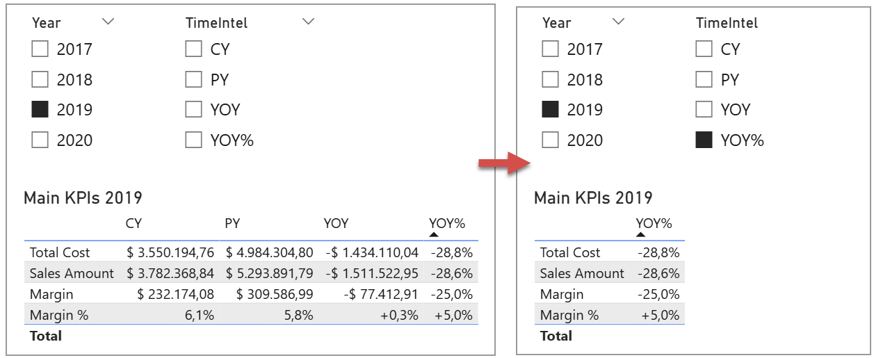
DAX UDF measures provide centralized code while keeping all the flexibility of independent measures

To replicate the behavior of the previous figure, it is necessary to build measures, field parameters, and dynamic measures. Let’s take a quick look at them. You will notice that some expressions can be simplified. The reason they are built this way is that they were automatically created with C# scripts that will be introduced later in the article.

// Field Parameter (slicer and matrix columns)
TABLE 'Parameter TimeIntel' =
    {
        ("CY", NAMEOF('Selection TimeIntel'[CY]), 0, "CY"),
        ("PY", NAMEOF('Selection TimeIntel'[PY]), 1, "PY"),
        ("YOY", NAMEOF('Selection TimeIntel'[YOY]), 2, "YOY"),
        ("YOY%", NAMEOF('Selection TimeIntel'[YOYPCT]), 3, "YOYPCT")
    }

// Rows Table
TABLE 'Selection baseMeasure' =
    {
        ("Margin", "Margin", 0),
        ("Margin %", "Margin %", 1),
        ("Sales Amount", "Sales Amount", 2),
        ("Total Cost", "Total Cost", 3)
    }

// YOYPCT semi-dynamic Measure
VAR __baseMeasure = SELECTEDVALUE( 'Selection baseMeasure'[baseMeasure Key] )
RETURN
    SWITCH(
        TRUE( ),
        __baseMeasure = "Margin %", [Margin % YOY%],
        __baseMeasure = "Margin", [Margin YOY%],
        __baseMeasure = "Sales Amount", [Sales Amount YOY%],
        __baseMeasure = "Total Cost", [Total Cost YOY%],
        BLANK( )
    )
, FormatString =
VAR __baseMeasure = SELECTEDVALUE( 'Selection baseMeasure'[baseMeasure Key] )
RETURN
    SWITCH(
        TRUE( ),
        __baseMeasure = "Margin %", "+0.0%;-0.0%;-",
        __baseMeasure = "Margin", "+0.0%;-0.0%;-",
        __baseMeasure = "Sales Amount", "+0.0%;-0.0%;-",
        __baseMeasure = "Total Cost", "+0.0%;-0.0%;-",
        ""
    )

// Measure example
Total Cost YOY% = Local.TimeIntel.YOYPCT( [Total Cost] )
DAX UDF function example
Local.TimeIntel.YOY =
    ( baseMeasure: ANYREF ) =>
    VAR ValueCurrentPeriod = Local.TimeIntel.CY( baseMeasure )
    VAR ValuePreviousPeriod = Local.TimeIntel.PY( baseMeasure )
    VAR Result = 
        IF( 
            NOT ISBLANK( ValueCurrentPeriod ) && NOT ISBLANK( ValuePreviousPeriod ), 
            ValueCurrentPeriod - ValuePreviousPeriod
        )
    RETURN
        Result

It’s hard to escape the filter context of a calculation group

Let’s now discuss another challenge you may face when using calculation groups. When a calculation item is part of the filter context, all measures are affected, and this creates certain challenges.

Creating a column chart with month-to-date sales seems like a quick win for calculation groups. However, things get tricky when the end user wants to hide dates with no sales for the active filters, because yes, measure-value filters in the filter pane are affected as well by the calculation item.

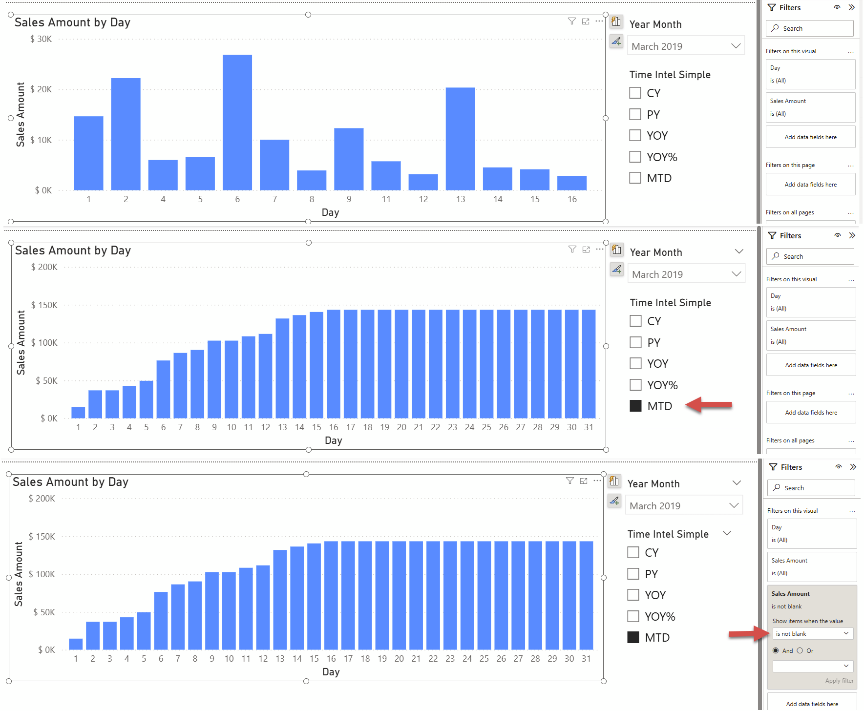
Calculation items also affect measures in the filter pane, therefore dates without sales remain visible

Solving this challenge using calculation groups implies having two versions of the same measure, one which will be modified by the calculation group and the other one which will not, for example “Sales Amount” and “Sales Amount NO CG”. But this workaround is painful to maintain and understand when you come back to the model months later.

Sales Amount NO CG = [Sales Amount]
MTD = 
IF(
    RIGHT( SELECTEDMEASURENAME(), 5 ) = "NO CG",  // If the name ends in "NO CG",
    SELECTEDMEASURE(),				              // don't modify the expression,
    CALCULATE(					                  // otherwise apply MTD filter
        SELECTEDMEASURE(),
        DATESMTD( 'Date'[Date] )
    )
)

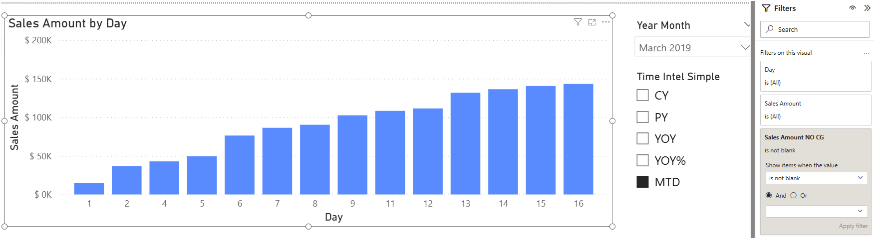
The workaround with calculation groups implies the duplication of measures only for this purpose and extra logic in the calculation item

Compare the previous workaround with the following chart implementation, with DAX UDF measures. You have both measures as separate entities, so you can use them however you see fit. One measure for Sales Amount, one measure for Sales Amount Month-to-Date. And Month-to-Date logic is still centralized in a DAX UDF.

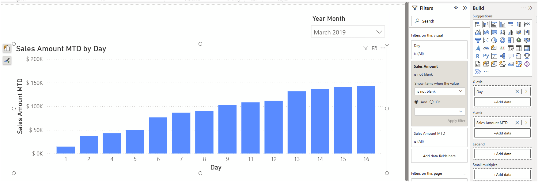
Using DAX UDF measures simplifies the implementation of this chart

Another simple use case that showcases the problem with calculation groups and filter context is the following one. Imagine you create a line chart showing current year (CY) and previous year (PY) sales over time. To do so, you use the base measure and the calculation group column in the legend, filtering the calculation items to show only CY and PY calc items. So far so good. Then you decide to add a tooltip to show both values along with year-over-year and year-over-year percent calculations. You set up the tooltip page, and it all seems to work fine until you test it and realize that the calculation items on the tooltip are being filtered, and only CY and PY remain visible.

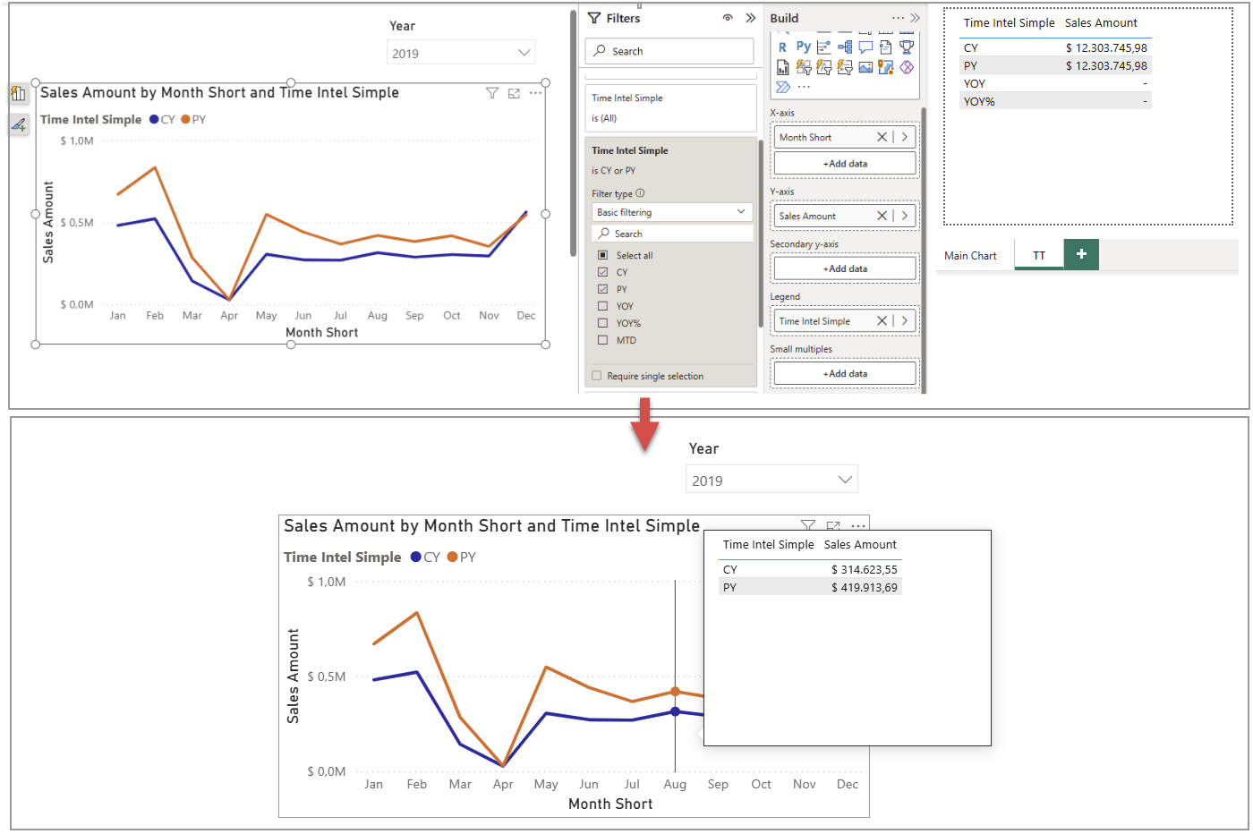
Due to the filter on the calculation group column in the filter pane, YOY and YOY% calculation items are not visible in the tooltip

The workaround is not simple, and I have written about it (here and here). I’m happier about the second article where basically, the idea is to remove the calculation group from the legend and filter pane and instead use the calculation group inside measures, to avoid filtering the calculation items in the tooltip.

In this example, “Time Intel Simple” is the calculation group with a column with the same name, while “PY” is the name of the calculation item.

Sales Amount PY (Calc Group Inside) =
    CALCULATE([Sales Amount], 'Time Intel Simple'[Time Intel Simple] = "PY")

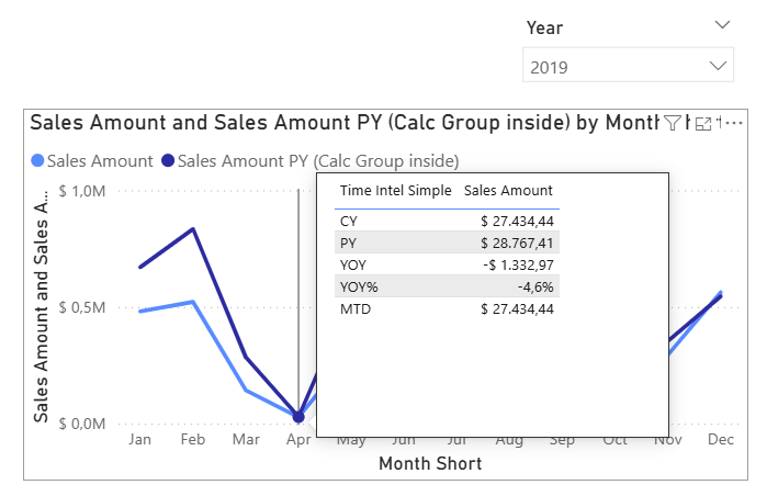
The workaround to avoid filtering the tooltip involves creating measures with the calculation item applied inside the DAX expression

Again, while possible, it’s complex, time consuming, and self-defeating since reducing the need to create measures is one of the main selling points of calculation groups. Furthermore, a potential danger of this workaround is that with such measures in the model, it is possible to build a visual where the same calculation item is applied twice, once through the filter context and once through the DAX expression. In such cases, the calculation item is only applied once, but this may not be what the developer expects and he or she may or may not realize what is happening.

Once again, let’s now compare the previous approach with working with DAX UDF measures. The calculation logic continues to be centralized, and yet, we don’t have to deal with undesired filter context issues. Just use the measures you want in the chart, and the ones you want in the tooltip. No extra steps are required.

Sales Amount CY = Local.TimeIntel.CY( [Sales Amount] )
Sales Amount PY = Local.TimeIntel.PY( [Sales Amount] )
Sales Amount YOY = Local.TimeIntel.YOY( [Sales Amount] )
Sales Amount YOY% = Local.TimeIntel.YOYPCT( [Sales Amount] )

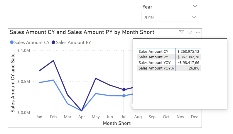
Using only measures and no calculation groups avoids undesired filtering in the tooltip

Creating the desired table

Let’s now discuss another challenge. When creating a table visual (or in fact a matrix) with calculation groups, there’s no flexibility in how elements are presented or even ordered. All current year measures will go together, then all previous year measures and so on. If the requirement is to show first some calculations on sales amount and then some calculations (same or different) for say, margin %, with calculation groups you are in trouble. As usual, there are workarounds (and I've written about them here), but they are neither intuitive nor easy to maintain.

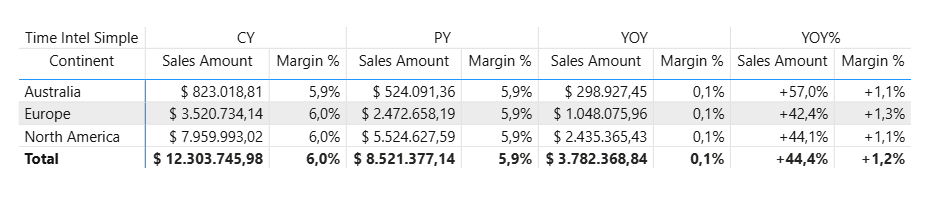
With time intelligence calculation groups, grouping columns by base measure or hiding certain combinations of base measure and calculation requires complex DAX expressions and/or separate calculation groups

If you have all the base measures, it’s possible to reach the desired outcome with one or two disconnected tables and a single measure. In this example we are just editing an expression generated by a script, leaving the combinations of base measures and calculations we want to see.

Custom Dynamic Measure for Chart = 
VAR __baseMeasure = SELECTEDVALUE( 'Selection baseMeasure'[baseMeasure Key] )
VAR __TimeIntel = SELECTEDVALUE( 'Selection TimeIntel'[TimeIntel Key] )
RETURN SWITCH(
    TRUE( ),
    __baseMeasure = "Margin %" && __TimeIntel = "CY", [Margin % CY],
    __baseMeasure = "Margin %" && __TimeIntel = "YOY", [Margin % YOY],
    __baseMeasure = "Sales Amount" && __TimeIntel = "CY", [Sales Amount CY],
    __baseMeasure = "Sales Amount" && __TimeIntel = "PY", [Sales Amount PY],
    __baseMeasure = "Sales Amount" && __TimeIntel = "YOY", [Sales Amount YOY],
    __baseMeasure = "Sales Amount" && __TimeIntel = "YOYPCT", [Sales Amount YOY%],

    BLANK( )
)

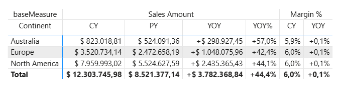
DAX UDF measures make implementing this type of chart easier while also maintaining logic centralized in a single place.

As we can see, having all the measures ready to use while keeping their code centralized brings unprecedented flexibility and control at the same time. You can either use the measures directly in whatever order or grouping the visual requires, mix them with measures from outside the time-intelligence set, or surface them through a field parameter or dynamic measures for end-user control.

Conditional Formatting

Conditional formatting is a dreaded challenge when working with calculation groups to the point that many Power BI developers are convinced that is just not possible and treat it as a limitation. When using a calculation group as columns in a matrix, it is difficult to conditionally format just one of the columns because in the UI it only offers to conditionally format the measure. Of course, this is the same behavior that you will get if you use any field to slice the data in columns, but it is with calculation groups when you want to configure different conditional formatting by visual column.

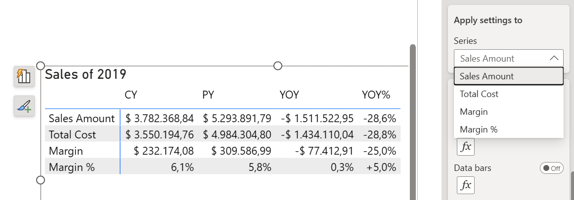
Conditional format is defined at the measure level so it’s not easy to specify for a single calculation item

The workaround is not straightforward and requires setting up a separate calculation group and a “twin measure”. Today there is no need to go down this path, but if you are curious, here you can read the article about it; this is one of the most popular articles of my blog, which tells how difficult this is to set up.

With DAX UDF measures, there’s no workaround to learn. You select the measure you want to format, and that’s it. Of course, if you want to use the same structure of the image and be able to set up the format by time calculation all at once, you will need to repackage your measures using semi-dynamic measures and field parameters, but don’t worry, we will see how to achieve that later in the article with C# scripts.

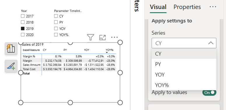
DAX UDF measures are the natural building blocks for dynamic measures and field parameters that allow more flexible reporting without cumbersome workarounds

Self-Service

As pointed out in the article by SQLBI, if the comparison is limited to DAX UDFs versus calculation groups, we can’t even start comparing them from a self-service perspective because DAX UDFs are not visible when consuming the model to build a report (though they can be used in DAX queries). However, here the comparison is between calculation group + base measures vs ready-made measures with each of their logic encapsulated in a DAX UDF.

DAX UDF measures are easier to use by end users because they don’t need to learn how to use a calculation group, think about the filter context created by the calculation group, and other aspects we saw in the previous sections (or even others we did not cover such as calculation group precedence). Calculation groups have their place in self-service to swap active relationships and other safe use cases where the shortcomings we have outlined do not apply. Beyond that, they should be avoided because the moment a user wants more, he or she needs to learn quite a few things about calculation groups to understand what is going on and use numerous workarounds along the way.

Performance

Finally, let’s very briefly discuss performance, even if this is not limited to time intelligence calculations and is beyond the scope of this article where we focus rather on usability. Performance is one of the weak aspects of calculation groups. No matter how you put it, calculation groups represent an important overhead that happens in query time.

In practice, DAX UDF measures perform as well as or better than calculation groups. Ricardo Rincon showed at a recent event how using a calculation group inside the visual would break DAX fusion whereas DAX UDFs do not, for simple filters like Color = “Red” or Country = “Germany”.

Efficiently working with DAX UDFs

Up to this point we have covered several scenarios where DAX UDF measures are more flexible and easier to use than calculation groups, but ‘the elephant in the room’ has not been addressed: how do you create all those measures in the first place?

When creating a measure, there are 6 elements you must or might want to configure: Base table, Display folder, Name, Expression, Format, and Description

In practice, if done manually, even maintaining a 100% homogeneous naming convention (let alone the other properties) is not easy. When working with DAX UDF measures, all these properties (and more, as we will see) can be defined based on the parameters metadata and the actual DAX UDF name. There’s no case-by-case decision to be made and having perfectly uniform measure definition has many advantages. Let’s see how Tabular Editor C# scripts can help us work efficiently with DAX UDFs.

This script will create measures for you

Create Measures From DAX UDFs.cs

As I published the day that DAX UDFs came out in public preview, I made a script that can automate measure creation (you can read it here).

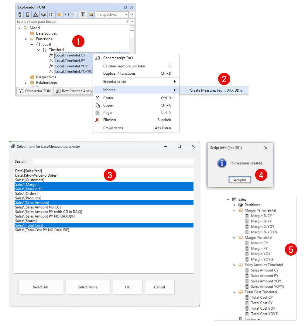
The script “Create Measures from DAX UDFs” can effortlessly create measures

Everything the script does can be done by hand, but it would just take much longer. To summarize the article, through different annotations in each DAX UDF you can define the template for the different properties of the resulting measure (Name, Display Folder, Format String, Base Table, and 2 annotations). Some elements can be hard-coded. For instance, any measure generated with a function to calculate year-over-year percent, will have a percent format regardless of the format of the base measure. Yet, for a year-to-date measure you might want to replicate whatever format the base measure had. To encode this logic in each of the properties, you can refer to some of the properties of the function parameters by using the parameter names with the following suffixes:

Now, rather than go in detail of the meaning of each suffix and how to use it, let’s see an example with a DAX UDF with a single measure parameter.

Example of extended configuration of a DAX UDF through annotations

baseMeasureFormatStringFull refers to the complete format string of the measure passed as baseMeasure parameter, in the example measure below: “$#,0;($#,0)”. baseMeasureFormatStringRoot would represent only the first part of the format string, “$#,0”.

Example of a parameter and corresponding output for the previous DAX UDF

All these parameter and suffix values can be used in a larger expression. For example, in a Year-Over-Year DAX UDF, as format string template you might want to use something like:

+baseMeasureFormatStringRoot;-baseMeasureFormatStringRoot;-

It is possible to execute the script while selecting multiple DAX UDFs and provide multiple values for each of the parameters, so for instance, creating all the time intelligence measures can be done in a single execution. If there are two or more parameters and two or more values are provided for each parameter, measures will be created for all possible combinations. I use this macro daily, in my daily work as a consultant. Here you can see the script in action:

This script will create the field parameter with extra fields

Create Field Parameter (with Properties).cs

This script has been shown in presentations but not properly introduced in an article. The need for this script became obvious when I started working with large amounts of DAX UDF measures produced by the previous script. End users had grown used to calculation groups and still wanted to swap the base measure while keeping the time intel calculations, or the other way around, keep the base measure but swap between actuals and YTD values.

Luckily for all of us, since calculation groups came out, other great things have happened to Power BI, including field parameters, which are great for swapping measures and columns in charts. When you create a field parameter in Power BI Desktop, though, the resulting calculated table only has three columns, the display name, the name of the field (measure or column) and the sort order.

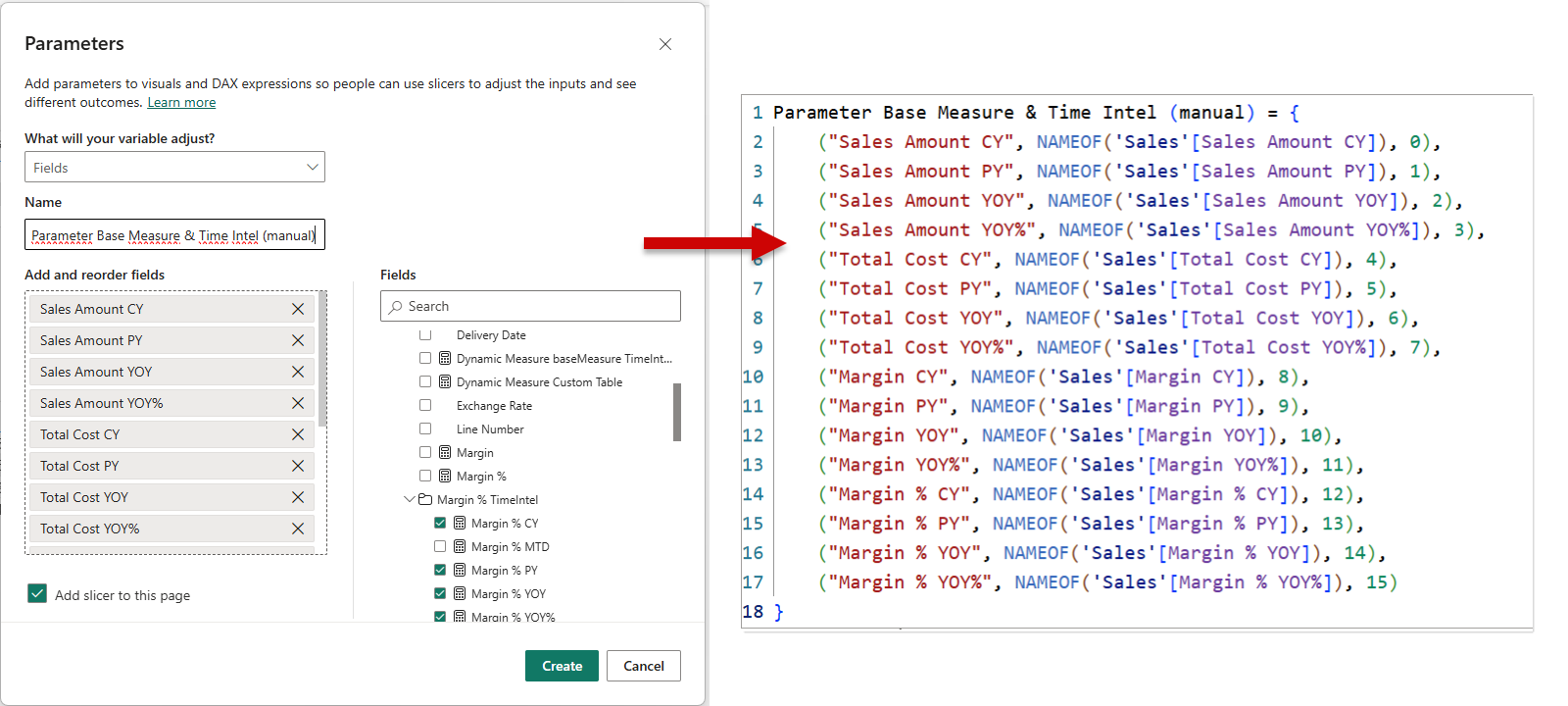
Field Parameters created through Power BI Desktop interface do not have columns to group by base measure or calculation.

If you want to group the different rows to easily filter them by some criteria such as base measure or calculation, it’s up to you to manually generate the columns editing the DAX expression or adding calculated columns.

You probably guess where this is going: with the C# script of this section, we can indeed create field parameters with the extra columns based on the Properties and PropertyNames annotations.

Here we can see the script in action:

To clarify the point, let’s see an example. When you select a group of measures like this:

The table view of the field parameter generated will look like this:

And the suggested name of the field parameter will be “Parameter baseMeasure TimeIntel”, which quickly identifies what this field parameter is about as well as keeping all field parameters together in the data pane with this naming convention.

This script will create dynamic and semi-dynamic measures for you

Create Dynamic Measure (with Properties).cs

Field parameters are great, but there are multiple places in a report where field parameters are not allowed, and other tools like Excel can’t consume field parameters at all. In these situations, you will need a dynamic measure, in other words, a measure that based on the value of one or more columns returns the value and format of different measures. For measures like the ones we just created, a dynamic measure can be very convenient, slicing by base measure and calculation you get the value with the right format, very close to what we had in calculation groups, and very convenient to build certain visuals that require a field inside the visual slicing by base measure or calculation.

Well, good news, this script will create this measure for you, along with the necessary disconnected tables with all the different values found in the Properties annotations of the selected measures. And not only that, at the same time it will create “semi-dynamic measures”, meaning, for example, a measure for each time intel calculation with the name of the calculation, that will return the right value when sliced by the base measure slicer.

Let’s see an example. Selecting all the measures created with the previous script, this macro will produce the following output:

• A dynamic measure in the same table as the first selected measure. The default name for this example is “Dynamic Measure baseMeasure TimeIntel”. It will pick up all the values from PropertyNames annotation making it clear what sort of dynamic measure it is. You might recognize the expression from an example earlier on the article. This is the expression as created by the script:

VAR __baseMeasure = SELECTEDVALUE( 'Selection baseMeasure'[baseMeasure Key] )
VAR __TimeIntel = SELECTEDVALUE( 'Selection TimeIntel'[TimeIntel Key] )
RETURN
    SWITCH(
        TRUE( ),
        __baseMeasure = "Margin %" && __TimeIntel = "CY", [Margin % CY],
        __baseMeasure = "Margin %" && __TimeIntel = "PY", [Margin % PY],
        __baseMeasure = "Margin %" && __TimeIntel = "YOY", [Margin % YOY],
        __baseMeasure = "Margin %" && __TimeIntel = "YOYPCT", [Margin % YOY%],
        __baseMeasure = "Margin" && __TimeIntel = "CY", [Margin CY],
        __baseMeasure = "Margin" && __TimeIntel = "PY", [Margin PY],
        __baseMeasure = "Margin" && __TimeIntel = "YOY", [Margin YOY],
        __baseMeasure = "Margin" && __TimeIntel = "YOYPCT", [Margin YOY%],
        __baseMeasure = "Sales Amount" && __TimeIntel = "CY", [Sales Amount CY],
        __baseMeasure = "Sales Amount" && __TimeIntel = "PY", [Sales Amount PY],
        __baseMeasure = "Sales Amount" && __TimeIntel = "YOY", [Sales Amount YOY],
        __baseMeasure = "Sales Amount" && __TimeIntel = "YOYPCT", [Sales Amount YOY%],
        __baseMeasure = "Total Cost" && __TimeIntel = "CY", [Total Cost CY],
        __baseMeasure = "Total Cost" && __TimeIntel = "PY", [Total Cost PY],
        __baseMeasure = "Total Cost" && __TimeIntel = "YOY", [Total Cost YOY],
        __baseMeasure = "Total Cost" && __TimeIntel = "YOYPCT", [Total Cost YOY%],
        BLANK( )
    )

• As you can see in the previous expression, it will generate a disconnected table for each of the values contained in the PropertyNames annotation. They are implemented as DAX calculated table, and the name starts with “Selection”, so they stay together in the data pane and don’t get mixed with the rest of the model tables. Each table has a field used for display that can be changed, the key field with the values expected by the dynamic measure (which must not be changed), and an order column to easily reorder display items if needed.

A similar table is built for baseMeasure as well.

• To get maximum flexibility, in each of the disconnected tables, semi-dynamic measures are created for each of the rows of the table. This means that instead of slicing by the ‘Selection TimeIntel’ table, you can use each of the measures instead. The code for “CY (dynamic)” measure looks like this:

VAR __baseMeasure = SELECTEDVALUE( 'Selection baseMeasure'[baseMeasure Key] )
RETURN
    SWITCH(
        TRUE( ),
        __baseMeasure = "Margin %", [Margin % CY],
        __baseMeasure = "Margin", [Margin CY],
        __baseMeasure = "Sales Amount", [Sales Amount CY],
        __baseMeasure = "Total Cost", [Total Cost CY],
        BLANK( )
    )

Where calculation groups are still the right answer

Calculation groups remain the right answer for use cases beyond time intelligence. The clearest one is changing active relationships in role-playing dimension scenarios — swapping order date for delivery date via USERELATIONSHIP, for example.

Calculation groups can also create otherwise impossible relationships with TREATAS (covered in this Esbrina article) or make filters behave in unconventional ways (see reversing a slicer selection).

Also, sometimes certain DAX optimizations may produce blanks where there should be values (or at least used to be this way). Calculation groups block many such optimizations and in certain edge cases can help you achieve the result you expect. SQLBI recognizes the issue here and I wrote about it in this Esbrina post.

Further recommended reading

• DAX UDFs parameters. When writing DAX UDFs, it’s important to specify if parameters are passed as a reference or as a value. Read about it in this article from SQLBI
• Save the scripts as macros, so you are always ready to use them (available in both TE2 and TE3). Read about the process in this Tabular Editor documentation article
• Field parameters are a thing on their own. Owen Auger wrote an excellent article about them

In conclusion

Well, this has been a rather long article, diving deep into calculation group usability issues and the scripts that make DAX UDFs a real alternative to them. Now, it is up to you to decide what you want to do. The scripts may look daunting for those who have never used scripts before, but there’s no need to understand each line of the code to run them; focus on the outputs, as they only create the same model objects you might create by hand. Test them and consider DAX UDF measures the next time you hit one of the calculation-group friction points discussed here. For the scenarios where calculation groups still serve well, keep using them. DAX UDF measures provide centralized code with the flexibility of independent measures, and Tabular Editor C# scripts can help write all the associated boilerplate DAX.