Optimizing semantic model size in Power BI and Fabric: a comprehensive guide

Key Takeaways

• Reducing the size of a semantic model improves performance, reduces cost, and keeps it below the limits of your Power BI / Fabric tenant: This is true irrespective of whether you use Fabric or Power BI / Direct Lake or import models. It’s therefore important that you invest in optimizing model size. This article presents you six patterns to do that.
• Simple optimizations limit the model to only what you need: Remove unnecessary columns and rows before attempting other optimizations, then reduce precision, split high cardinality columns like DateTime, and select appropriate data types. You can also disable unnecessary attribute hierarchies via IsAvailableInMDX.
• Advanced optimizations tailor your model design to your scenario: User-defined aggregations reduce VertiPaq memory by moving detailed data to DirectQuery while keeping aggregated data in Import mode. This shifts cost from memory to query time; it must be carefully evaluated. You can also split a large semantic model into smaller, subject-oriented models to reduce peak memory usage per model.
• Advanced compression techniques can situationally be worth investigating: Examples include optimizing for run-length encoding, can further reduce the memory footprint when structural optimizations have already been applied.

This summary is produced by the author, and not by AI.

Understanding model size optimization

This article is the second in a series on optimizing semantic model memory in Microsoft Fabric. In the first article, we explained that:

• Memory refers to the size that your semantic model takes on disk in Power BI and Microsoft Fabric.
• There’s hard memory limits for Power BI semantic models; if you exceed these limits, then you experience query and refresh errors.
• Fabric enforces memory per semantic model, and full refresh requires headroom.
• You can measure where memory is consumed by using the VertiPaq Analyzer by SQLBI in Tabular Editor 3 or DAX Studio, or in Fabric notebooks (where it’s called the “Memory Analyzer”).

In this article, we shift from understanding to action. Instead of analyzing limits and failure modes, our focus pivots to practical modeling decisions that measurably and meaningfully reduce semantic model size. The goal is not to blindly apply tricks, but to understand what you can do, why each pattern works, and how to validate its impact.

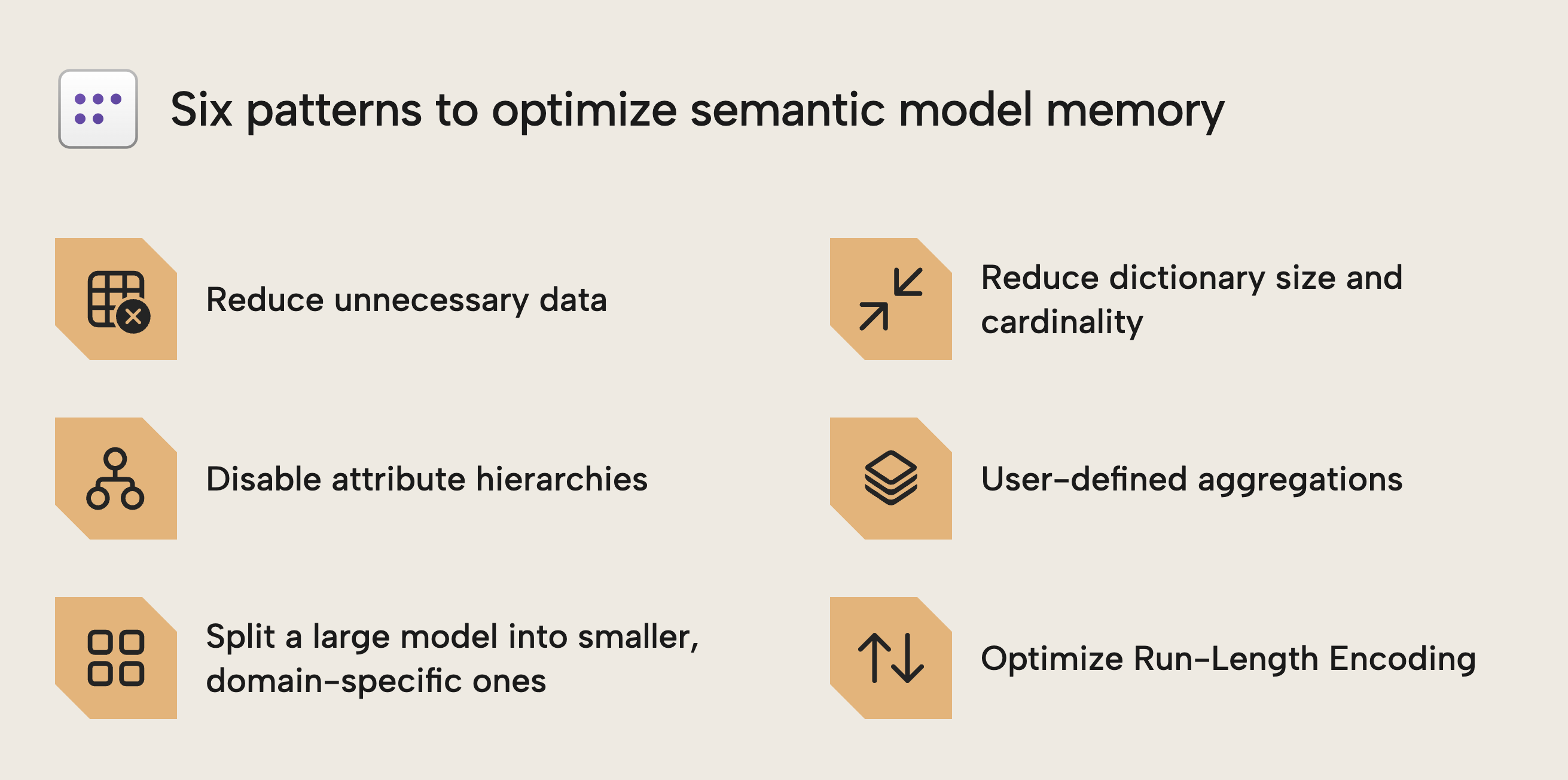
The following six patterns and techniques are concrete design choices that reduce semantic model memory usage. Each pattern builds on the same principles introduced in Part 1:

These six patterns are presented in the section, below.

Pattern one: Reduce unnecessary data

Reducing unnecessary data is the simplest and most effective way to lower semantic model size. The principle is straightforward: reduce the width (columns) and height (rows) of your tables to only what is required for reporting and analysis. You should always apply this pattern for every model, both during design of a new model, but also optimization of an existing one. This sounds obvious, but in practice it requires discipline.

It’s common to include columns in a semantic model “just in case” someone needs it. It’s also common to import years of detailed history because it’s available in the source. A question you should ask is: does this data serve a concrete reporting requirement today? If not, it is probably better left out. You can always add it later, if and when it’s needed.

The goal is to include only the data required for analysis. For example, is ten years of detailed transactional data necessary to calculate YTD and YoY? In many cases, current and previous year are sufficient at detailed grain, while older data can be aggregated. Removing rows through filters or incremental refresh policies can significantly reduce model size without affecting business value. Hybrid tables are another solution,

Columns are often the bigger problem. Audit fields, GUIDs, technical identifiers, and rarely used attributes frequently consume disproportionate memory, especially when they have high cardinality. Once such columns are used in measures or report visuals, removing them becomes difficult. It is therefore safer to identify and exclude them early during model design and development, rather than to remove them later, when they might be already used in some obscure visual or reporting process.

Why this works

This pattern is the simplest to do and understand; if you exclude or remove a column or table, then it’s not contributing to the model size. To reiterate, the difficulty here isn’t in the implementation. It comes in deciding what to remove, the implications for your model and report designs, and how you’ll fulfill inevitable user requests when they do need that information.

How to reduce unnecessary data

To implement this pattern, you first want to define the narrowest range of data that you need to include in the model (via inclusion criteria applied to filters and table/column selection). This is relevant not only for date ranges with filtering, but any category. Once you exclude columns, don’t forget to make sure that you aggregate your data, too.

To help you figure out which columns you want to incorporate in your semantic model. What you want to focus on is which columns take up the most size, and identify whether you can remove these columns, outright. Consider the highlighted columns in the example from the previous article:

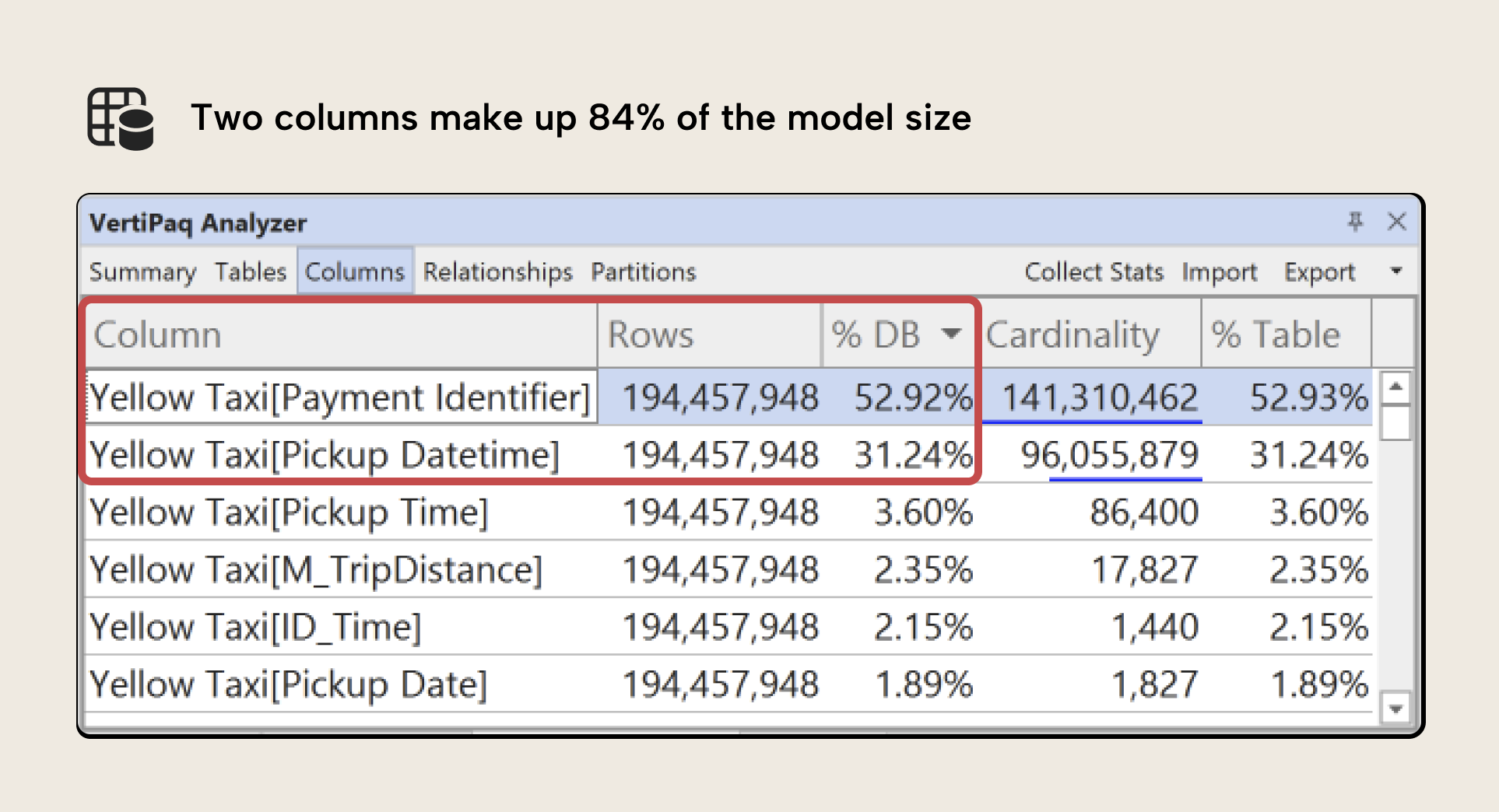
These two columns account for 84% of the model size. It’s likely that we need the Pickup Datetime field (but can optimize it, further), but Payment Identifier is a key field we might remove, perhaps replacing with an aggregate Number of Payments if necessary.

If you’re refactoring an existing model, then you might want to know which columns aren’t used in calculations and relationships. Tabular Editor’s Best Practice Analyzer includes a rule to detect unused columns in the model. While this does not account for report usage, it provides a useful starting point for identifying obvious candidates for removal.

But let’s say that you have identified some large columns, but you do need them in your model; you can’t remove them. What then?

Pattern two: Reduce cardinality and dictionary size

In the previous example, we can remove the Payment Identifier column, but not the Pickup Datetime column. Both columns are large because they have a high cardinality, which refers to the number of unique rows in that column. You can see this in the example screenshot; a cardinality of 96M means that there’s 96M unique rows in the Pickup Datetime column, for instance.

High-cardinality columns are one of the most common causes of large semantic models. VertiPaq builds a dictionary of unique values for each column and stores encoded references to that dictionary. When a column has many unique values (especially near-unique values) the dictionary becomes large, and compression efficiency drops.

To understand this better, consider the following diagram:

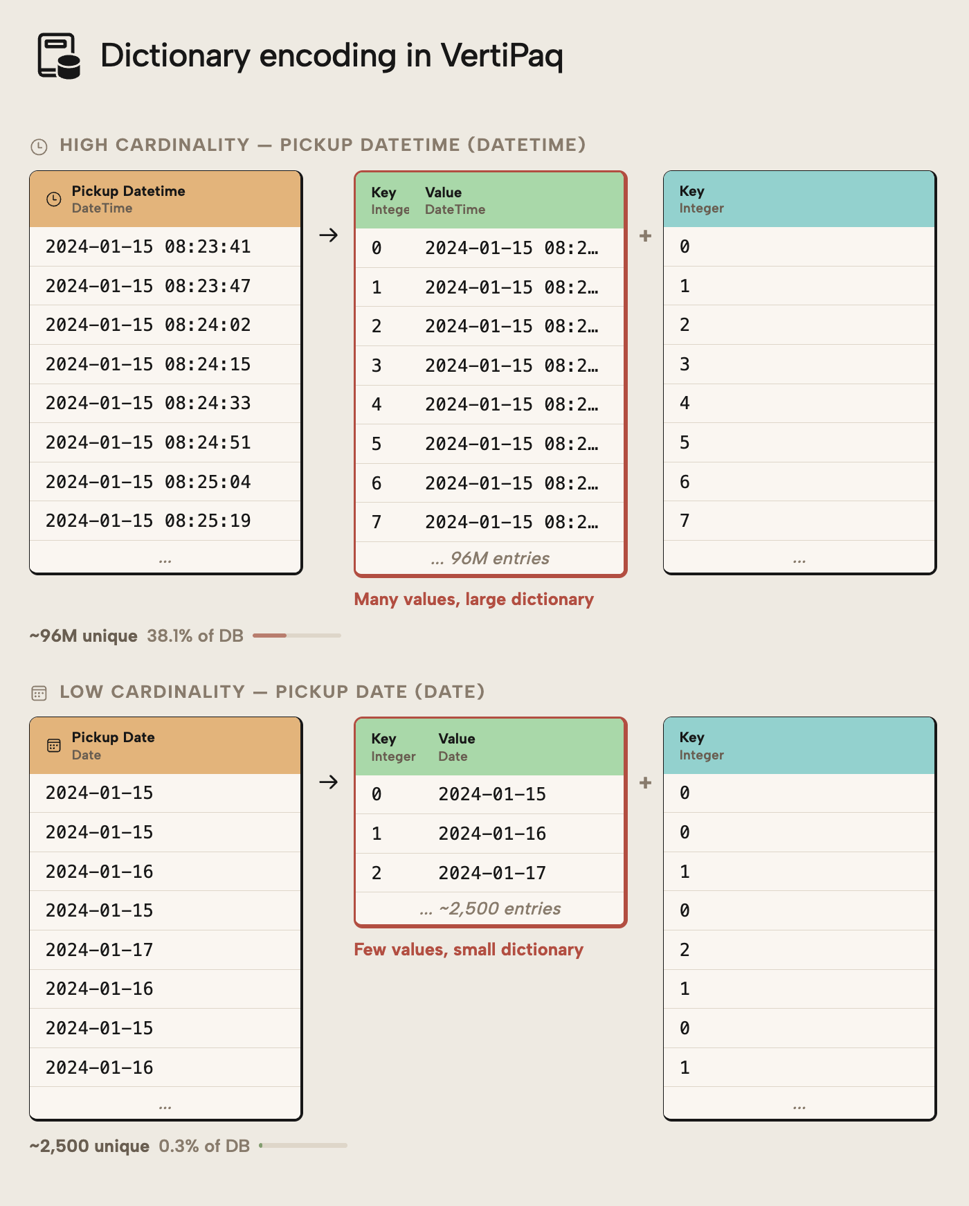
Pickup DateTime has 96M unique values; the dictionary is therefore very large and the column can’t be well compressed by VetiPaq. In contrast, if we have the date alone (such as when splitting date and time into separate columns), there’s only 2,500 unique values. The column is much more effectively compressed and the model is smaller size… even though the number of rows did not change at all.

A DateTime column is a very common example of this. Often, columns like this serve as a technical identifier in the source system. From a reporting perspective, only the Date might be required. By either trimming the time altogether or splitting Date and Time into separate columns, the semantic model size can drop dramatically… anecdotally, we at Tabular Editor have seen numerous cases where a simple operation like this reduce model size by more than 50%!

Therefore, a second way to reduce model size is by transforming the data to limit the number of unique values. Think of it like this: reducing unnecessary columns removes entire structures from the model, while reducing cardinality shrinks the columns that must remain.

Why this works

Dictionary size is directly tied to the number of unique values in a column. By reducing precision, splitting columns, or selecting more appropriate data types, you reduce cardinality and increase compression efficiency. The result is often large memory savings from relatively small modeling changes.

How to reduce cardinality

Implementing this pattern involves any technique that can reduce the number of unique values in a high-cardinality column. To reiterate, splitting a DateTime column into separate Date and Time columns is often beneficial. The Date column typically has low cardinality and compresses well. The Time column can often be reduced to minute-level precision and linked to a Time-of-Day dimension if needed. If a combined value is required for reporting, it can be recreated as a measure rather than stored as a high-cardinality column.

This is true not only for DateTime columns, but also other identifiers. Consider an example where a utilities company needs the identifier of customers’ electricity meters in reports. This field could be a long alphanumeric string with near-unique cardinality, with values like SE-GBG-E-2019-0045821, where segments encode region, meter type, installation year, and a sequential number:

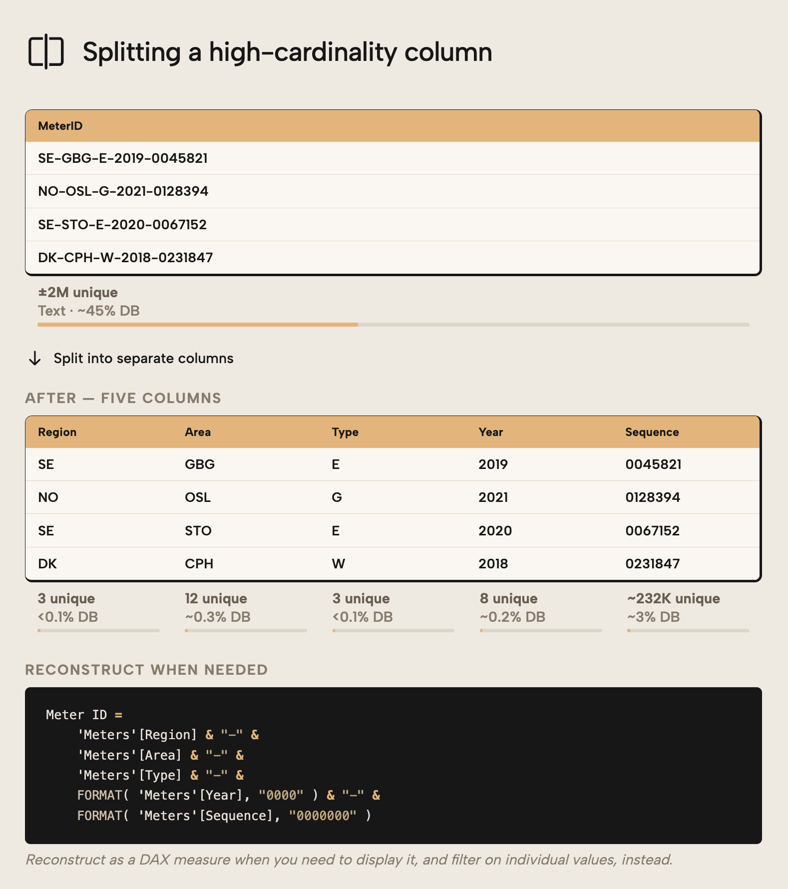
Stored as a single column, the dictionary must hold one entry per meter; ±2M total which make up 45% of the model size in the example. Splitting it into separate columns (Region, Type, Year, and Sequence Nr) replaces one high-cardinality column with several low-cardinality columns that compress efficiently than the composite string identifier. Filters can still be applied to individual columns, while the full identifier can still be reconstructed as a DAX measure when you need to display it in a report or query.

Another common improvement is choosing appropriate data types. Avoid floating-point types (Double, Single, Float) for values that require exact precision, especially financial amounts. Use Fixed Decimal (Currency) where appropriate and Integers for identifiers and counts. The precision of floating-point types increases memory usage and can introduce rounding inconsistencies.

Further, you want to avoid using String data types for numerical columns. When you use a string data type, the column will not be able to optimally compress because of how the model encodes the data. The following diagram depicts a few examples for you to better understand how data types affect column (and therefore model) size:

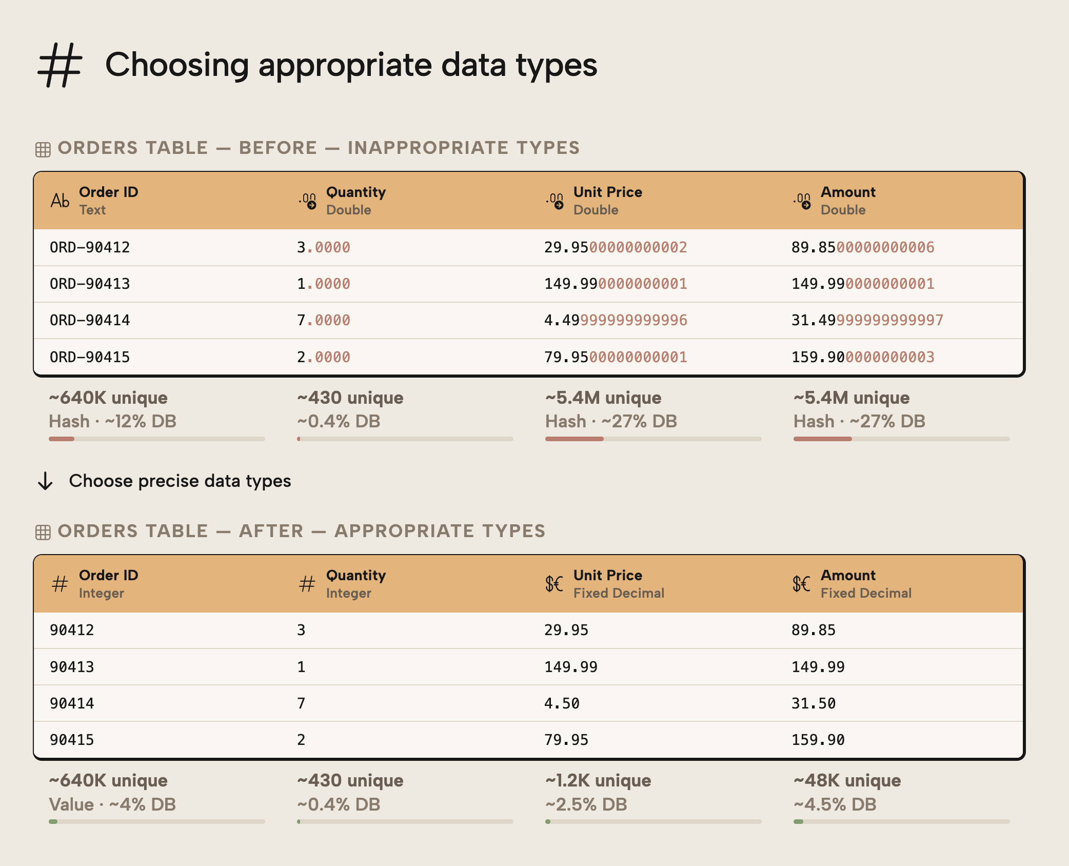
The examples above demonstrate the following:

• OrderID becomes smaller because an integer column can use VALUE encoding for better compression in VertiPaq.
• Qty doesn’t become smaller because the number of unique values doesn’t change. Changing the data type from Double to Integer has no effect on cardinality or dictionary size, so the column isn’t made smaller.
• Unit Price and Amount have too much decimal precision. Changing to a Fixed Decimal data type reduces the precision, which reduces the number of unique values. It’s important that you make sure that you only reduce precision in a way that won’t meaningfully affect the values of calculations that use these columns.

This pattern focuses on reducing column size via data transformations. However, a simple property switch can in some cases have the same effect.

Pattern three: Disable unnecessary attribute hierarchies

The previous two patterns focused on the data itself… removing columns you don't need and shrinking the ones you choose keep. However, the VertiPaq engine doesn't just store your data, but also builds supporting structures around it. Those structures consume memory, too.

By default, Power BI creates what's called an attribute hierarchy for every column in your model. An attribute hierarchy is a piece of metadata that allows certain client tools (most notably Excel Pivot tables like in Analyze-in-Excel) to browse and interact with that column. Under the hood, Excel doesn't speak DAX; it uses an older query language called MDX, and attribute hierarchies are what make MDX queries work. If you've ever dragged a field onto a PivotTable axis, you've used an attribute hierarchy to query the data.

The problem is that these structures are generated for every column in your model, including columns that will never appear in a pivot table… surrogate keys, technical identifiers, GUIDs, and columns used only inside DAX measures. Your users might not even be using Analyze-in-Excel, in which case these hierarchies are literally just wasted space with cost and no value. Particularly for high-cardinality columns, this overhead is sizable.

The impact is clearly visible in VertiPaq Analyzer:

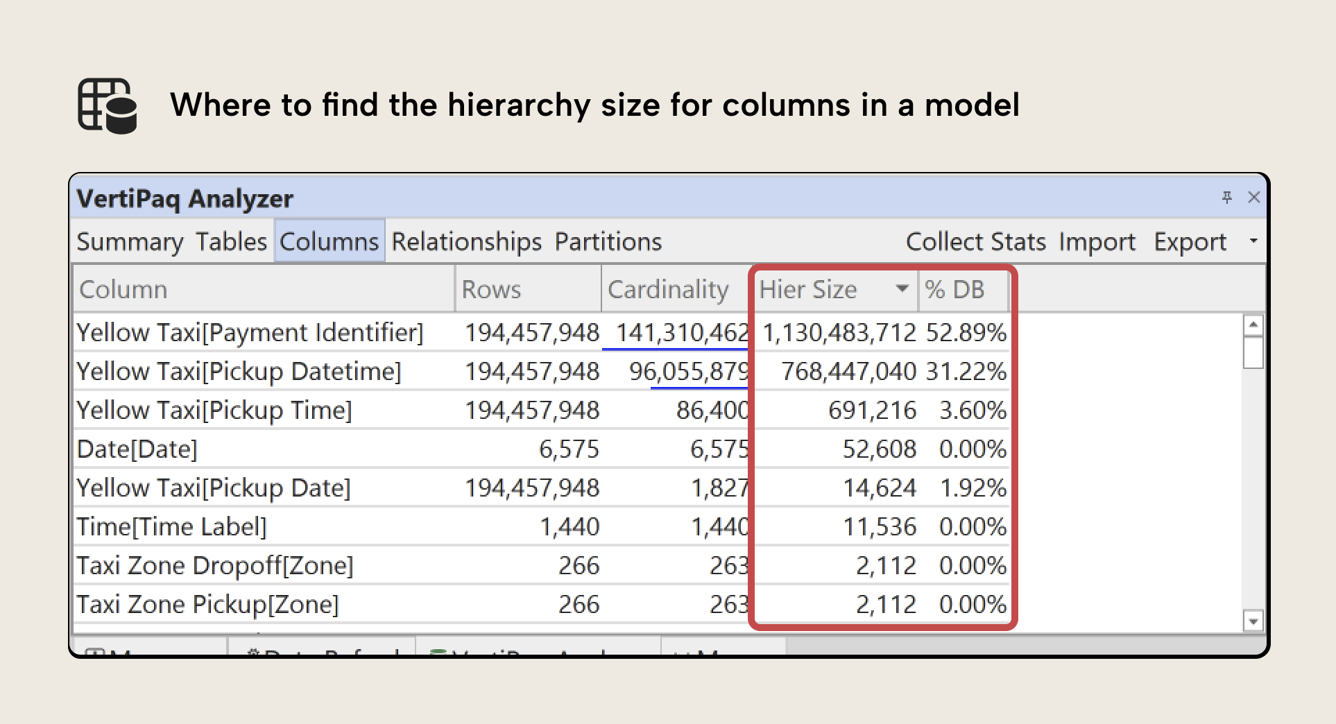
In the example above, the Payment Identifier column has a hierarchy size of approximately 1.1 GB, out of a total column size of 7.7 GB. That is the hierarchy overhead alone.

Why this works

Disabling IsAvailableInMDX removes unused hierarchy structures and reclaims the associated memory. If you disable IsAvailableInMDX, then Hier Size comprises only the explicit hierarchies that you create yourself.

How to remove unwanted or unused attribute hierarchies

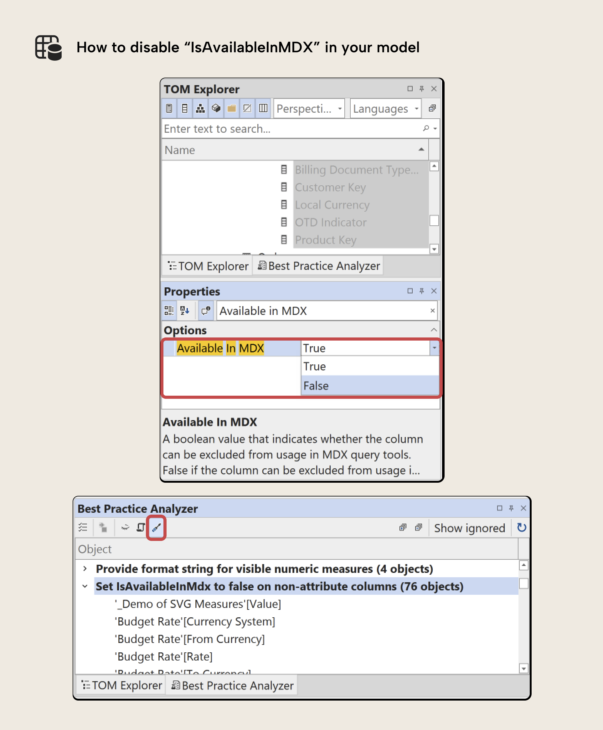
Setting the property IsAvailableInMDX to false on a column prevents the attribute hierarchy from being created. The column itself remains fully functional… it just stops generating MDX metadata that nobody uses. You can do this in Tabular Editor via the “Properties Pane” when selecting one or more columns, using Semantic Link Labs in a Fabric notebook, or in the TMDL view of Power BI Desktop, which requires that you write out the createOrReplace TMDL script for every column where you want to make this change.

Bonus tip: Use Detail Rows Expression to preserve controlled access

A concern concern with disabling attribute hierarchies is whether users lose the ability to see detail. For instance, if you disable IsAvailableInMDX in the Order Number and Order Line Number columns, what if users want this data in their pivot table? There’s an easy solution for this using Detail Rows Expressions in DAX.

In Excel, users can double-click an aggregated PivotTable cell to "drill through" to the rows behind it. When no Detail Rows Expression is defined, that drillthrough generates an MDX query that returns every column from the underlying fact table. This includes surrogate keys, GUIDs, and technical identifiers, etc… columns with little analytical value that can produce enormous intermediate result sets and spike CU consumption on Fabric. Not good!

Defining a Detail Rows Expression for a table replaces that bad default behavior. Instead of an MDX-generated column dump, the drillthrough executes a DAX query based on your Detail Rows Expression that returns only the columns you specify via SELECTCOLUMNS. You control what users see, in what order, and with what column names. Related dimension attributes can be pulled in via RELATED, giving users a curated, readable result set rather than a raw fact table export.

This is a better default for most models. Users can still access detail intentionally through drillthrough, but they can no longer accidentally drag a million-row identifier column onto a PivotTable axis… a scenario that generates expensive MDX queries and freezes their workbook..

Thus, this technique allows you to:

• Disable unnecessary attribute hierarchies
• Prevent high-cardinality columns from being used directly in PivotTable rows or columns
• Return only the columns required for detailed analysis
• Improve performance by avoiding unnecessarily wide result sets

A full step-by-step implementation guide is provided in the Detail Rows Expressions tutorial published on the Tabular Editor documentation.

So far, we’ve discussed several basic patterns that help you eliminate or optimize the size of columns in your table. Those patterns can be completed quickly; often, in minutes. The next patterns are more advanced, since they involve design or architectural changes to your semantic model.

Pattern four: User-defined aggregations to isolate high-cardinality detail

Sometimes you cannot remove or reduce high-cardinality detail columns. They may be required for reconciliation, auditing, operational verification, etc. In those cases, a technique called user-defined aggregations provide an alternative to keeping all details fully imported into memory.

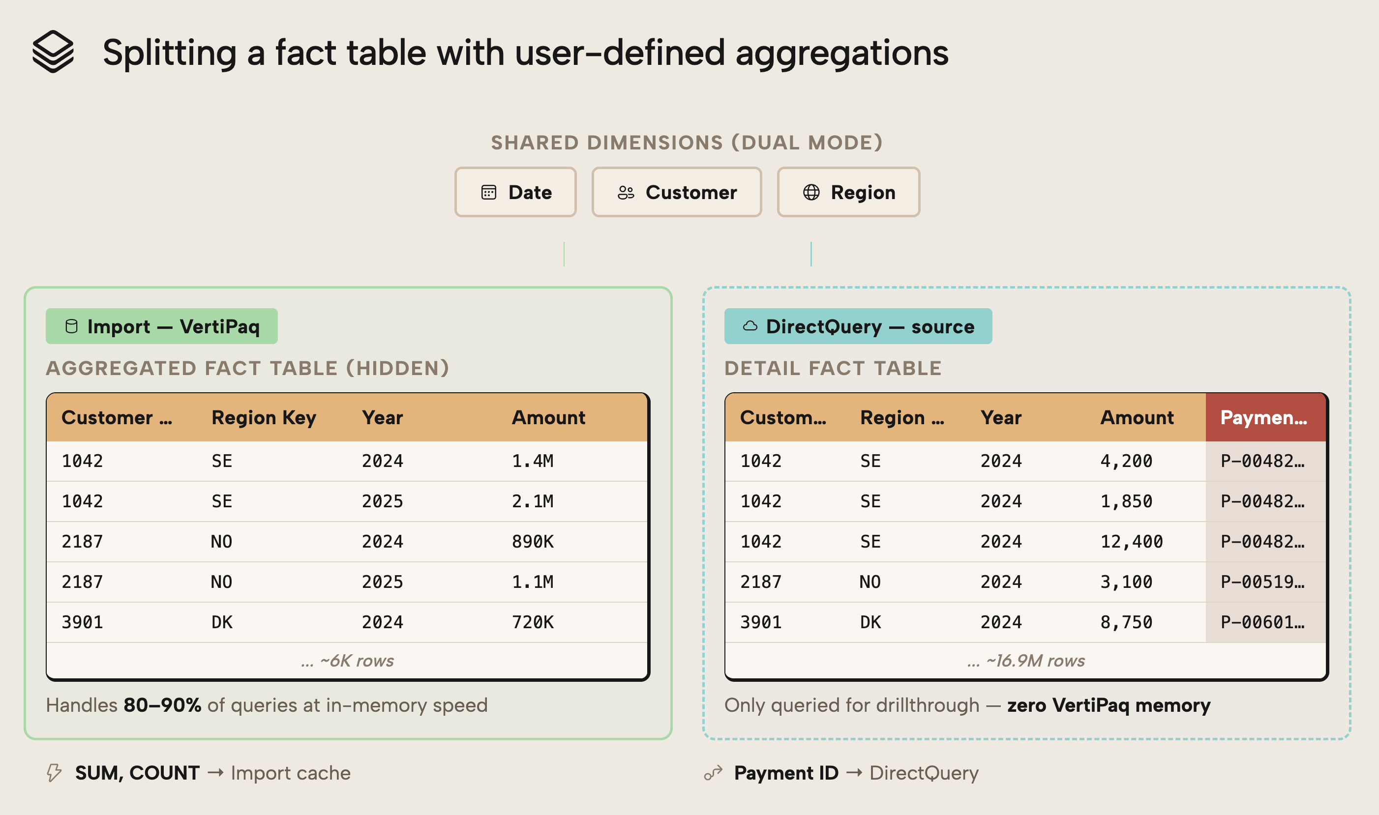
User-defined aggregations let you split a fact table into two logical layers within a composite model: a smaller, aggregated Import table that handles most reporting queries, and a detailed DirectQuery table that retains the high-cardinality columns you can't afford to import. Power BI routes queries to whichever layer can answer them:

• Aggregated queries should hit the fast in-memory cache by default. This is your standard import table that has the aggregate data.

Detail-level drillthrough hits DirectQuery; against the source… but only when necessary. This is a detailed DirectQuery “shadow” table, containing high-cardinality columns.

By moving high-cardinality detail columns out of the import tables, you remove their dictionary, data, and hierarchy structures from VertiPaq storage. The imported portion of the model becomes significantly smaller and more compression-efficient.

The detailed DirectQuery table still exists, but it does not consume VertiPaq memory as an imported column does. Memory usage is therefore reduced at the cost of query-time access when detail is required.

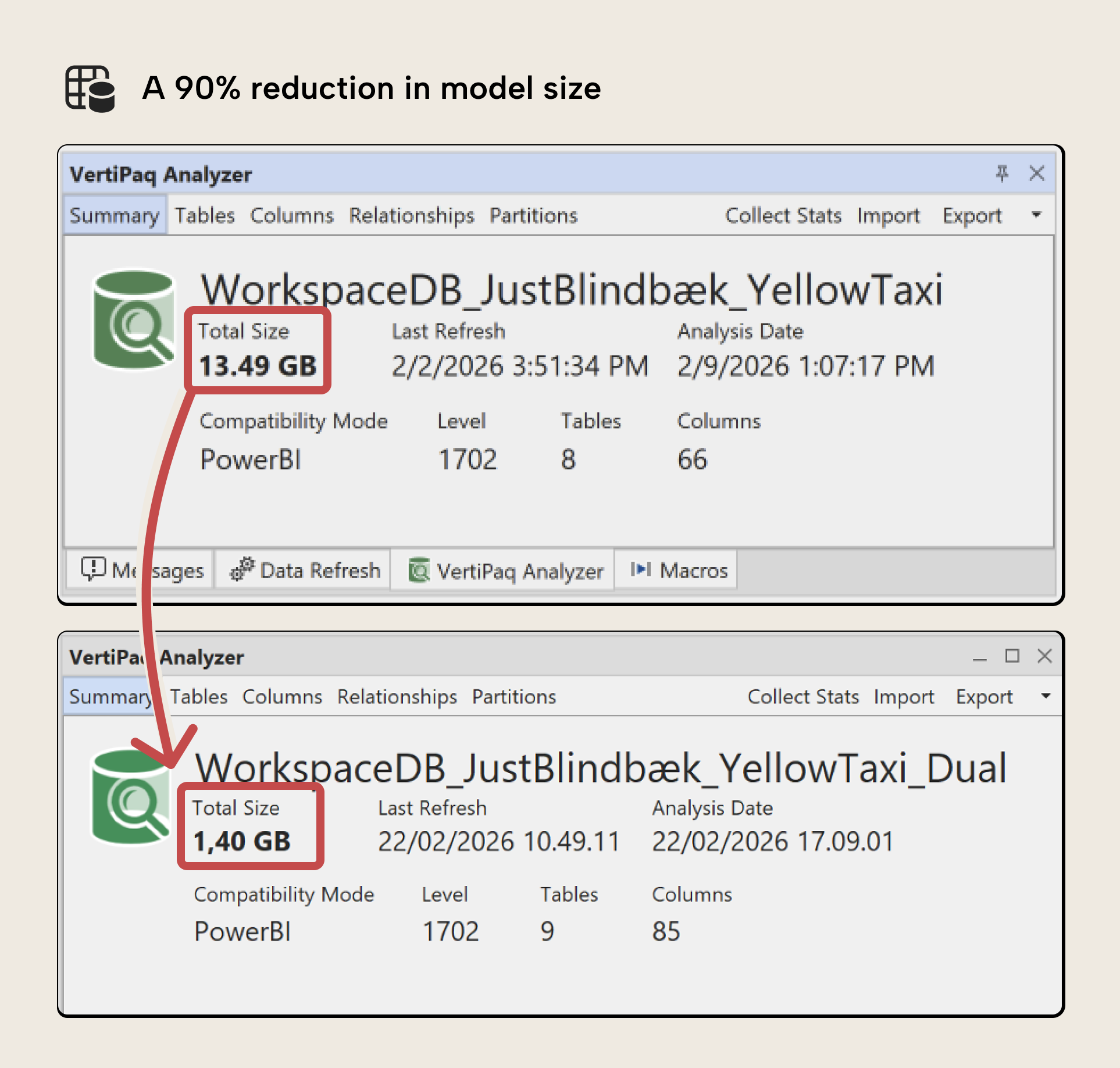
As the following image demonstrates, you can reduce the size of a model by a lot with this pattern; 90% in this example:

This pattern is especially effective when:

• 80–90% of reporting relies on aggregated measures
• Detailed rows are accessed infrequently
• High-cardinality columns dominate model size
• Detailed data is typically accessed with strong filters, allowing source system indexes to efficiently retrieve relatively small result sets

To avoid accidental performance degradation:

• Hide DirectQuery detail columns from report users
• Provide guidance on when detailed access is appropriate
• Combine this pattern with Detail Rows Expression where relevant

Why this works

VertiPaq memory is consumed by imported data structures. By keeping only aggregated data in Import mode and moving granular, high-cardinality columns to DirectQuery, you reduce dictionary and segment storage while preserving access to full detail when needed.

How to implement user-defined aggregations

User-defined aggregations are a complex, multi-step process to set up in Power BI Desktop or Tabular Editor. You need to consider various factors that depend on your data and scenario. Therefore, implementation details are intentionally omitted here, as a full tutorial is provided separately in the Tabular Editor documentation.

Bonus tip: Working with storage mode

When you use user-defined aggregations, you change your model from an import storage mode to a composite model that comprises multiple storage modes (having table partitions that are import and partitions that are DirectQuery). As we mentioned in the previous article, you can also opt for a DirectQuery or Direct Lake storage mode, but changing the storage mode has significant consequences, and isn’t a solution for memory optimization in Power BI or Fabric:

• DirectQuery shifts the cost from memory to query and results in worse performance.
• Direct Lake still requires memory optimization and has additional technical factors to consider.

In a nutshell, this pattern takes an import model and turns it into a composite model where aggregate data uses in-memory data, and detailed data uses DirectQuery. However, you still have one model. The next pattern discusses what happens if you split up the model into multiple, smaller ones, while keeping them “in sync”.

Pattern five: Split it up into smaller models (the master model pattern)

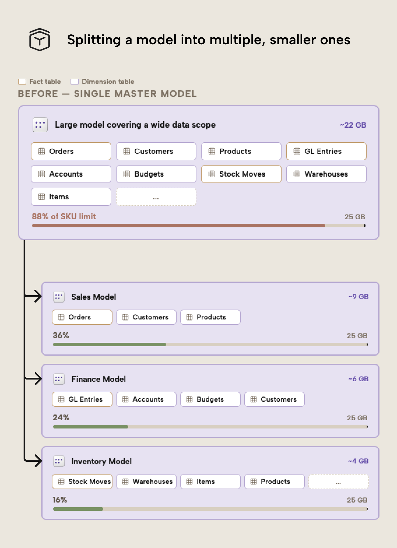
As we discussed in the first article of this series, Fabric enforces memory limits per semantic model. A large, multi-domain “master” model therefore concentrates all memory pressure in a single resource-consuming artifact. Splitting that model into smaller, subject-oriented semantic models can therefore reduce the memory footprint per model, which helps to avoid hitting SKU limits.

Instead of a single large model covering Sales, Finance, Inventory, and Operations, in this pattern, you create separate models for each domain. Each model then contains only the tables and columns required for its analytical scope. This reduces the amount of imported data within each semantic model.

The result is not necessarily a smaller overall data footprint across the organization, but it is smaller per semantic model. Because Fabric capacity limits are enforced at the model level, this distinction is critical.

Note that this isn’t just a memory optimization technique. It can also improve governance and maintainability by:

• Aligning semantic models with organizational ownership
• Isolating deployments per domain
• Simplifying security management
• Allowing independent release cycles

These benefits might even justify the design choice if memory pressure or performance isn’t a pain or primary driver.

A note on architectural implications

A Power BI report can connect to only one semantic model at a time. Splitting models therefore introduces constraints. Cross-domain reporting becomes more complex and may require:

• A lightweight “management” model containing shared KPIs.
• Conformed dimensions across models.
• Use of other items, like dashboards that pin visuals from multiple reports, or even notebooks that consume and present data from multiple models.

This pattern works best when domains are naturally separated and users rarely need to combine analysis across them. This pattern also increases operational complexity and typically requires a code-first deployment strategy (e.g., CI/CD pipelines using Tabular Editor, Fabric CLI and Fabric CI/CD, as well as other, similar supportive tools). Manual, report-first workflows don’t exactly scale well when multiple semantic models must remain synchronized.

Why this works

Because memory limits are enforced per semantic model, distributing data across multiple models reduces peak memory consumption per model. This can prevent refresh failures and allow lower SKUs (or even Power BI Pro) to be used more effectively.

How to split and maintain a model into multiple smaller ones

This is obviously a significant design decision that should not be taken lightly. Special precautions must be taken to ensure that the smaller models remain “in sync”, such as using a “master model pattern”. A detailed implementation guide, including scripting examples in Tabular Editor, is available in the Tabular Editor documentation.

Pattern six: Optimize Run-Length Encoding (RLE)

Run-Length Encoding (RLE) is one of the compression mechanisms used by VertiPaq. While dictionary encoding often receives the most attention, RLE can deliver meaningful memory savings when data is structured to take advantage of it.

RLE works by compressing consecutive repeated values. The longer the “runs” of identical values in a column segment, the more efficient the compression becomes. If values alternate frequently, compression efficiency decreases.

This means that data ordering and column design can affect the memory footprint.

When fact tables are sorted so that similar values are grouped together — for example, by low-cardinality columns or natural grouping keys — columns with repeating values can achieve longer runs within segments. This increases compression efficiency and reduces storage size. You can understand this better with the following diagram:

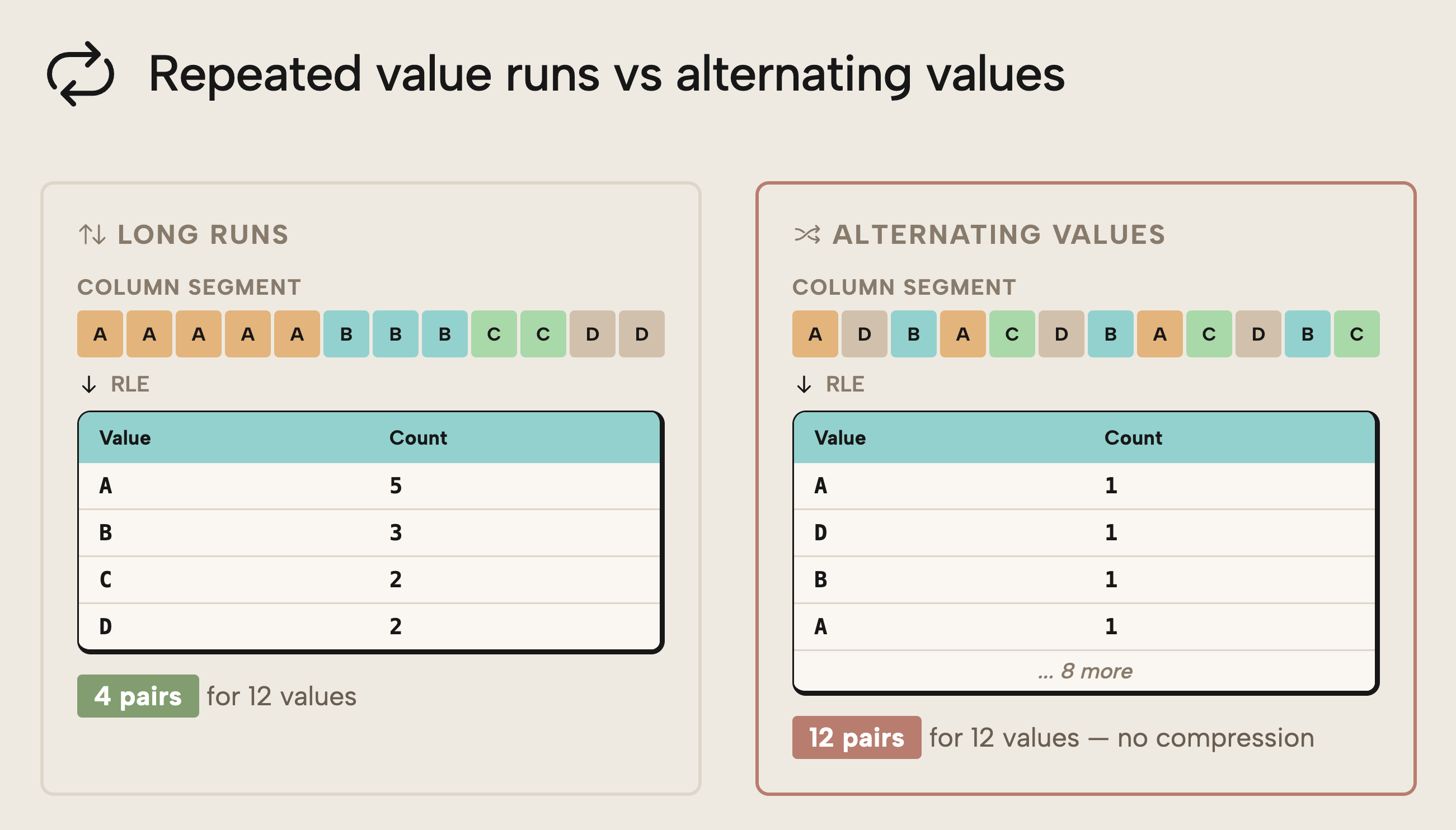
On the left is depicted a sorted column with long runs of the same value. This results in RLE with a total of 4 pairs for 12 values in this hypothetical example; good compression. In contrast, on the right, suboptimal sorting means that we can’t “compress” this column to few pairs.

Since this is a complex technical topic, here’s another (still simple) example, this time from the SpaceParts dataset:

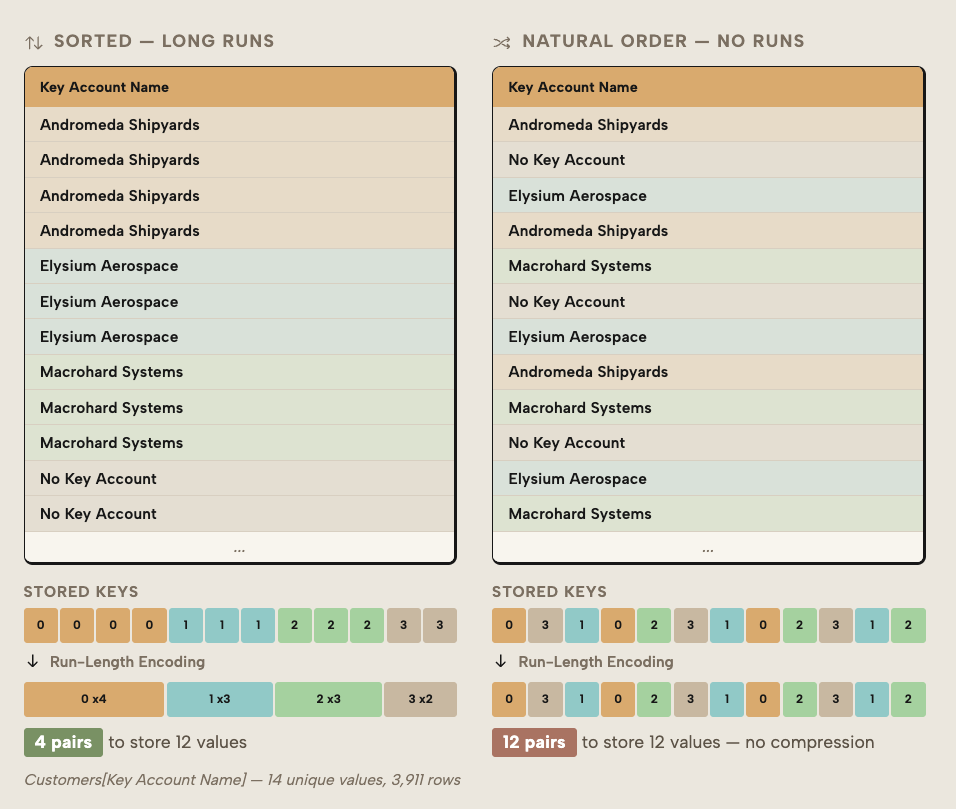
In short, you can see that the optimal sorting results in better RLE, and therefore smaller column sizes.

The effect is not theoretical. In a practical example shared by Jonathan Otykier, optimizing for RLE reduced the size of a fact table by approximately 16% without removing any data. The savings came solely from improved compression behavior.

You want to consider this pattern in the following scenarios:

• When large fact tables dominate memory usage
• When other column-level reductions have already been applied
• When the model cannot be split further
• When you want to optimize without changing business semantics

Why this works

VertiPaq stores data in column segments. When identical values appear consecutively within those segments, RLE can store them compactly as value + count instead of repeated entries. Structuring data to maximize these runs increases compression efficiency and reduces overall memory footprint.

How to implement RLE optimization

Optimizing RLE involves modifying sort order or sometimes partitioning (if you have multiple partitions) of your data.

Wrapping up

So far in this article series, we have explained what semantic model memory is, why it’s important to optimize, and how you can measure it. In this article, we guide you through six patterns – both basic and advanced – to help you optimize your models:

• Reduce unnecessary data
• Reduce unnecessary cardinality and dictionary size
• Disable unnecessary attribute hierarchies
• Leverage user-defined aggregations
• Apply the “master model pattern”
• Optimize run-length encoding (RLE)

In the next article of this series, we continue guiding you through optimization with a focus on optimizing semantic model refresh.

Further recommended reading

• Import modeling data reduction techniques (Microsoft Learn). Official guidance on reducing model size through column and row elimination, grain selection, and data type choices.
• VertiPaq Analyzer (SQLBI). Detailed explanation of how to inspect model size and interpret dictionary, data, and hierarchy structures.
• IsAvailableInMDX in SSAS Tabular (Chris Webb). Clear explanation of how disabling attribute hierarchies affects memory and Excel PivotTables.
• Controlling drillthrough in Excel PivotTables (SQLBI). Deep dive into Detail Rows Expression and drillthrough behavior.
• User-defined aggregations (Microsoft Learn). Official documentation on implementing aggregations in Power BI and composite models.
• Run-Length Encoding optimization example (Jonathan Otykier). Practical example demonstrating measurable model size reduction through RLE optimization.

In conclusion

Optimizing the size of the semantic model in Fabric is not about applying a single technique or blindly following best practices. Rather, you must consider your scenario, measure memory to inform decisions, and then apply deliberate design choices where they matter most to get the best results. Doing so will ensure that you get the most from your semantic models while keeping cost and performance well under control.